Ethoscopy
Ethoscopy user manual
- Getting started
- Metadata design
- Loading the data
- Behavpy
- Behavpy - Circadian analysis
- Behavpy - Hidden Markov Model
- Jupyter tutorials
- Tutorial 1 — Overview: working with ethoscope data
- Tutorial 2 — HMM: hidden behavioural states
- Tutorial 3 — Circadian analysis
- Tutorial 5 — catch22 feature extraction
- Tutorial 6 — Exporting to hctsa (MATLAB)
- Paper companion notebook — Jones et al.
Getting started
Installing ethoscopy as a docker container with ethoscope-lab (recommended).
The ethoscope-lab docker container is the recommended way to use ethoscopy. A docker container is a pre-made image that will run inside any computer, independent of the operating system you use. The docker container is isolated from the rest of the machine and will not interfere with your other Python or R installations. It comes with its own dependencies and will just work. The docker comes with its own multi-user jupyterhub notebook so lab members can login into it directly from their browser and run all the analyses remotely from any computer, at home or at work. In the Gilestro laboratory we use a common workstation with the following hardware configuration.
CPU: 12x Intel(R) Xeon(R) CPU E5-1650 v3 @ 3.50GHz
GPU: Intel(R) Xeon(R) CPU E5-1650 v3 @ 3.50GHz
Hard drive: 1TB SSD for OS, 1TB SSD for homes and cache, 7.3 TB for ethoscope data
Memory: 64GB
The workstation is accessible via the internet (behind VPN) so that any lab member can login into the service and run their analyses remotely. All the computational power is in the workstation itself so one can analyse ethoscope data from a tablet, if needs be.
What's in the latest image (ggilestro/ethoscope-lab:1.2)
- JupyterHub 5.4.0 · Python 3.10 kernel · R kernel with rethomics (behavr, ggetho, damr, sleepr, zeitgebr, scopr)
ethoscopy 2.0.5pre-installed; tutorial datasets (overview_data.pkl,circadian_data.pkl, etc.) already baked into the package directory, soget_tutorial('overview')works out of the box without a separate download step- Flexible authentication: shared-password (dummy), GitHub, Google, GitLab or Keycloak/OIDC — selected via a
.envfile at run time (see Authentication below)
Follow the instructions below to install the ethoscope-lab docker container on your machine.
Quick start with docker compose (recommended)
The ethoscopy repo ships a docker-compose.yml plus .env.*.example templates. On a machine that has Docker Engine with the compose plugin installed:
# Grab just the Docker/ directory (sparse-checkout keeps the rest of the repo off disk)
git clone --depth=1 --filter=blob:none --sparse https://github.com/gilestrolab/ethoscopy.git
cd ethoscopy
git sparse-checkout set Docker
cd Docker
# Pick an authentication method and write its settings to .env
cp .env.dummy.example .env # shared password — simplest
# or
cp .env.keycloak.example .env # Keycloak / generic OIDC
# or .env.github.example / .env.google.example / .env.gitlab.example
# Edit .env — at minimum set DUMMY_PASSWORD, ALLOWED_USERS, ADMIN_USERS
# (for OAuth, set OAUTH_CLIENT_ID / _SECRET / _CALLBACK_URL instead)
# Optional overrides at the top of .env:
# JUPYTER_HUB_TAG=5.4.0
# ETHOSCOPE_LAB_TAG=1.2
# UID=1000 GID=1000 # must match ownership of /mnt/homes and /mnt/cache
# Adjust docker-compose.yml's volumes: section so the three host paths point at
# places that actually exist on your box:
# - /mnt/ethoscope_data/results → /mnt/ethoscope_results (ro, your .db files)
# - /mnt/ethoscope_data/ethoscope_metadata → /opt/ethoscope_metadata
# - /mnt/homes → /home (per-user homes)
# - /mnt/cache → /home/cache (shared scratch)
docker compose up -d
The service is then exposed on port 8082 of the host (the docker-compose.yml maps 8082:8000 by default — change that line if you need a different host port). Point a browser at http://your-host:8082/.
Manual docker run (when you don't have compose)
The image can also be started directly. The simplest invocation, for a single-user trial on Linux, looks like this:
# Optional. Update the system to the latest version. You may want to restart after this.
sudo pamac update
# install docker
sudo pacman -S docker
# start the docker service
sudo systemctl enable --now docker
# download and run the ethoscope-lab docker container
# the :ro flag means you are mounting that destination in read-only
sudo docker run -d -p 8000:8000 \
--name ethoscope-lab \
--volume /ethoscope_data/results:/mnt/ethoscope_results:ro \
--restart=unless-stopped \
ggilestro/ethoscope-lab:1.2
Installation on Windows or MacOS makes sense if you have actual ethoscope data on those machines, which is normally not the case. If you go for those OSs, I won't provide detailed instruction or support as I assume you know what you're doing.
On MacOS
Install the docker software from here. Open the terminal and run the same command as above, e.g.:
sudo docker run -d -p 8000:8000 \
--name ethoscope-lab \
--volume /path/to/ethoscope_data/:/mnt/ethoscope_results:ro \
--restart=unless-stopped \
ggilestro/ethoscope-lab:1.2
On Windows
Install the docker software from here. After installation, open the window terminal and issue the same command as above, only replacing the folder syntax as appropriate. For instance, if your ethoscope data are on z:\ethoscope_data and the user data are on c:\Users\folder use the following:
sudo docker run -d -p 8000:8000 \
--name ethoscope-lab \
--volume /z/ethoscope_data:/mnt/ethoscope_results:ro \
--restart=unless-stopped \
ggilestro/ethoscope-lab:1.2
Storing user data on the machine, not on the container (recommended)
ethoscope-lab runs on top of a JupyterHub environment, meaning that it supports organised and simultaneous access by multiple users. Users have their own credentials and their own home folder. With the default .env.dummy.example settings, the demo user is ethoscopelab with password ethoscope, and each user's work lives in /home/<username>. In the minimal examples above, /home/<username> is stored inside the container, which is not ideal — you lose everything on a container recreate. A better solution is to mount the host's home folders at /home inside the container. In the example below, we use /mnt/my_user_homes:
sudo docker run -d -p 8000:8000 \
--name ethoscope-lab \
--volume /ethoscope_data/results:/mnt/ethoscope_results:ro \
--volume /home:/mnt/my_user_homes \
--restart=unless-stopped \
ggilestro/ethoscope-lab:1.2
Make sure your local home location contains a folder for each user (e.g.
/mnt/my_user_homes/ethoscopelab) with correct ownership — by default the container expects UID/GID1000:1000.
Any folder in /mnt/my_user_homes is then accessible to the corresponding user inside ethoscope-lab. In our lab we sync those using owncloud (an open-source Dropbox clone) so that every user has their files automatically synced across all their machines.
Authentication
The image supports five authentication methods, selected at startup via environment variables (typically a .env file consumed by docker compose):
| Method | When to use | .env template |
|---|---|---|
| Dummy | Small teams on a trusted network | .env.dummy.example |
| Keycloak / OIDC | Institutional SSO (production) | .env.keycloak.example |
| GitHub OAuth | Team gated by a GitHub organisation | .env.github.example |
| Google OAuth | Gated by a Google Workspace domain | .env.google.example |
| GitLab OAuth | Team on a GitLab instance | .env.gitlab.example |
Full instructions — including adding users, promoting admins, switching methods without data loss, and troubleshooting tokens — live in Docker/README_AUTH.md in the ethoscopy repo.
AUTHENTICATOR_CLASS=dummy
DUMMY_PASSWORD=pick-a-strong-password
ALLOWED_USERS=alice,bob,charlie,ethoscopelab
ADMIN_USERS=alice
Adding users without OAuth (rare)
If you're running the minimal docker run setup without an .env file and need to add a local user, you can drop into the container and create one the traditional way — this matches what ALLOWED_USERS already does automatically for compose deployments:
#enter a bash shell of the container
sudo docker exec -it ethoscope-lab /bin/bash
#create the username and home folder
useradd myusername -m
#set the password for the newly created user
passwd myusername
The user will then be able to login into Jupyter and work out of /home/myusername.
Persistent user credentials (legacy)
If you prefer to manage Linux-level credentials on the host rather than via .env or OAuth (for example, when you've inherited an older ethoscope-lab deployment), you can bind-mount /etc/passwd, /etc/shadow and /etc/group from the host into the container. This is the old approach; OAuth is now the recommended way to persist identities across image upgrades. An example:
sudo docker run -d -p 8000:8000 \
--name ethoscope-lab \
--volume /mnt/data/results:/mnt/ethoscope_results:ro \
--volume /mnt/data/ethoscope_metadata:/opt/ethoscope_metadata \
--volume /mnt/homes:/home \
--volume /mnt/cache:/home/cache \
--restart=unless-stopped \
-e VIRTUAL_HOST="jupyter.lab.gilest.ro" \
-e VIRTUAL_PORT="8000" \
-e LETSENCRYPT_HOST="jupyter.lab.gilest.ro" \
-e LETSENCRYPT_EMAIL="giorgio@gilest.ro" \
--volume /mnt/secrets/passwd:/etc/passwd:ro \
--volume /mnt/secrets/group:/etc/group:ro \
--volume /mnt/secrets/shadow:/etc/shadow:ro \
--cpus=10 \
ggilestro/ethoscope-lab:1.2
The last three --volume lines indicate the location of the user credentials. This configuration allows to maintain user information even when upgrading ethoscope-lab to newer versions.
Troubleshooting
If your Jupyter starts but hangs on the following image

It means that the ethoscopelab user does not have access to its own folder. This most likely indicates that you are running the container with a mounted home directory, but the ethoscope home folder is either not present or does not have read/write access for UID/GID 1000:1000 (the default inside the image — configurable via UID/GID in .env).
Install ethoscopy in your Python space
Ethoscopy is on github and on PyPi. You can install the latest stable version with pip3.
pip install ethoscopy
As of version 2.0.5, the required dependencies are:
Python >= 3.10
numpy >= 2.0
pandas >= 2.2.2
plotly >= 5.22
seaborn >= 0.13
hmmlearn >= 0.3.2
pywavelets >= 1.6
astropy >= 6.1
tabulate >= 0.9
colour >= 0.1.5
nbformat >= 5.10
Tutorial data
Starting with ethoscopy 2.0.5, the six tutorial pickle files (~36 MB total, dominated by overview_data.pkl at ~31 MB) are no longer bundled with the PyPI wheel — pip install ethoscopy ships code only. The tutorial notebooks fetch the datasets on demand with a single one-time call:
import ethoscopy as etho
etho.download_tutorial_data() # idempotent — skips files already on disk
By default this populates ~/.cache/ethoscopy/tutorial_data/, which is user-writable on every platform (no root or sudo needed). After that, get_tutorial('overview'), get_tutorial('circadian') and get_HMM('M'|'F') work as shown in the tutorial notebooks.
Lookup order. At load time, ethoscopy checks three locations in this order:
<site-packages>/ethoscopy/misc/tutorial_data/— dev / editable installs and theethoscope-labDocker image (which pre-populates it at build time, see below).$ETHOSCOPY_TUTORIAL_DATA_DIRif set — useful for shared clusters where one admin-maintained copy serves many users.~/.cache/ethoscopy/tutorial_data/— the default fordownload_tutorial_data().
The canonical URLs live at github.com/gilestrolab/ethoscopy/tree/main/src/ethoscopy/misc/tutorial_data. Place the six *.pkl files in any of the three locations above if you prefer to download manually.
ethoscope-lab users don't need to do anything. The Docker image (
ggilestro/ethoscope-lab:1.2and later) runsdownload_tutorial_data(dest_dir=package_tutorial_data_dir())during build, so the pickles are already present in the image. JupyterHub users can run the tutorials without any download step.
Metadata design
What is the metadata?
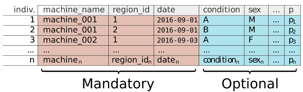
The metadata is a simple .csv file that contains the information to (1) find and retrieve the data saved to a remote server and (2) to segment and transform the data to compare experimental conditions. I would recommend recording as many experimental variables as possible, just to be safe. Each row of the .csv file is an individual from the experiment. It is mandatory to have at least the following columns: 'machine_name', 'region_id', and 'date' with date in a YYY-MM-DD format. Without these columns the data cannot be retrieved.
Top tips.
- Make the metadata exhaustive. Record everything just encase you need information in the future.
- Once you've finished all your replicates, put them in the same
csvfile with a column "replicate" to identify them. It's easier than loading them separately. - Make your metadata files straight away, as soon as you start your experiment. Time will erode the little details!
Loading the data
Setting up
To begin you need three paths saved as variables:
- the path to the metadata
.csvfile - the full path (including folder) the ftp location (eg: ftp://myethoscopedata.com/results/)
-
the path of a local folder to save downloaded
.dbfiles (if your .db files are already downloaded on the same machine running ethoscopy, then this will be the path to the folder containing them)
import ethoscopy as etho
# Replace with your own file/sever paths
meta_loc = 'USER/experiment_folder/metadata.csv'
remote = 'ftp://ftpsever/auto_generated_data/ethoscope_results'
local = 'USER/ethoscope_results'
# This will download the data remotely via FTP onto the local machine
# If your ethoscopy is running via ethoscope-lab on the same machine
# where the ethoscope data are, then this step is not necessary
etho.downlaod_from_remote_dir(meta_loc, remote, local)
download_from_remote_dir - Function reference
This function is used to import data from the ethoscope node platform to your local directory for later use. The ethoscope files must be saved on a remote FTP server and saved as .db files, see the Ethoscope manual for how to setup a node correctly.https://www.notion.so/giorgiogilestro/Ethoscope-User-Manual-a9739373ae9f4840aa45b277f2f0e3a7
This only needs to be run if like the Gilestro lab you have all your data saved to a remote ftp sever. If not you can skip straight to the the next part.
Create a modified metadata DataFrame
This function creates a modified metadata DataFrame with the paths of the saved .db files and generates a unique id for each experimental individual. This function only works for a file structure locally saved to whatever computer you are running and is saved in a nested director structure as created by the ethoscopes, i.e.
'LOCAL_DIR/ethoscope_results/00190f0080e54d9c906f304a8222fa8c/ETHOSCOPE_001/2022-08-23_03-33-59/DATABASE.db'
For this function you only need the path to the metadata file and the path the the first higher level of your database directories, as seen in the example below. Do not provide a path directly to the folder with your known .db file in it, the function searches all the saved data directories and selects the ones that match the metadata file.
meta_loc = 'USER/experiment_folder/metadata.csv'
local = 'USER/ethoscope_results' # remember to just provide the path up to the directory where the individual ethoscope files are saved
meta = etho.link_meta_index(meta_loc, local)Load and modify the ethoscope data
The load function takes the raw ethoscope data from its .db format and modifies it into a workable pandas DataFrame format, changing the time (seconds) to be in reference to a given hour (usually lights on). Min and max times can be provided to filter the data to only recordings between those hours. With 0 being in relation to the start of the experiment not the reference hour.
data = etho.load_ethoscope(meta, min_time = 24, max_time = 48, reference_hour = 9.0)
# you can cache the each specimen as the data is loaded for faster load times when run again, just add a file path to a folder of choice, the first time it will save, the second it will search the folder and load straight from there
# However this can take up a lot of memory and it's recommended to save the whole loaded dataset at the end and to load from this each time. See the end of this page
data = etho.load_ethoscope(meta, min_time = 24, max_time = 48, reference_hour = 9.0, cache = 'path/ethoscope_cache/')
Additionally, an analysing function can be also called to modify the data as it is read. It's recommended you always call at least max_velocity_detector or sleep_annotation function when loading the data as it generates columns that are needed for the analysis / plot generating methods.
from functools import partial
data = etho.load_ethoscope(meta, reference_hour = 9.0, FUN = partial(etho.sleep_annotation, time_window_length = 60, min_time_immobile = 300))
# time_window_length is the amount of time each row represents. The ethoscope can record multiple times per second, so you can go as low as 10 seconds for this.
# The default for time_window_length is 10 seconds
# min_time_immobile is your sleep criteria, 300 is 5 mins the general rule of sleep for flies, see Hendricks et al., 2000.
Ethoscopy has 2 general functions that can be called whilst loading:
- max_velocity_detector: Aggregates variables per the given time window, finding their means. Sleep_annotation uses this function before finding sleep bouts, so use this when you don't need to know the sleep bouts.
- sleep_annotation: Aggregates per time window and generates a new boolean column of sleep, as given by the time immobile argument.
sleep_annotation - Function reference
Ethoscopy also has 2 functions for use with AGO or mAGO ethoscope module (odour delivery and mechanical stimulation):
- stimulus_response: Finds the interaction times and then searches a given window post interaction for movement.
- stimulus_prior: A modifcation of stimulus_response, the function finds all interaction times and their response whilst retaining all the previous variables information in a given time window. I.e. if the window is 300, all 300 seconds worth of data will be retained prior to the second when the stimulus is given.
stimulus_response - Function reference
stimulus_prior - Function reference
Saving the data
Loading the ethoscope data each time can be a long process depending on the length of the experiment and number of machines. It's recommended to save the loaded/modified DataFrame as a pickle .pkl file. See here for more information about pandas and pickle saves. The saved behavpy object can then be loaded in instantly at the start of a new session!
# Save any behavpy or pandas object with the method below
import pandas as pd
df.to_pickle('path/behapvy.pkl') # replace string with your file location/path
# Load the saved pickle file like this. It will retain all the metadata information
df = pd.read_pickle('path/behapvy.pkl')
Behavpy
About
Behavpy is the default object in ethoscopy, a way of storing your metadata and data in a single structure, whilst adding methods to help you manipulate and analyse your data.
Metadata is crucial for proper statistical analysis of the experimental data. In the context of the Ethoscope, the data is a long time series of recorded variables, such as position and velocity for each individual. It is easier and neater to always keep the data and metadata together. As such, behavpy class is a child class of Pandas dataframe, the widely used data table package in python, but enhanced by the addition of a metadata as a class variable. Both the metadata and data must be linked by a common unique identifier for each individual (the 'id' column), which is automatically done if you've loaded with Ethoscopy (If not see the bottom of the page for the requirements for creating a behavpy object from alternative data sources).
The behavpy class has variety of methods designed to augment, filter, and inspect your data which we will go into later. However, if you're not already familiar with Pandas, take some time to look through their guide to get an understanding of its many uses.
Initialising behavpy
To create a behavpy object you need matching metadata and data. To match they both need to have an id column that has linked/same id's in each. Don't worry, if you downloaded/formatted the data using the built in ethoscopy functions shown previously they'll be in there already.
import ethoscopy as etho
# You can load you data using the previously mentioned functions
meta = etho.link_meta_index(meta_loc, remote, local)
data = etho.load_ethoscope(meta, reference_hour = 9.0, FUN = partial(etho.sleep_annotation, time_window_length = 60, min_time_immobile = 300))
# Or you can load then from a saved object of your choice into a pandas df,
# mine is a pickle file
meta = pd.read_pickle('users\folder\experiment1_meta.pkl')
data = pd.read_pickle('users\folder\experiment1_data.pkl')
# to initialise a behavpy object, just call the class with the data and meta as arguments. Have check = True to ensure the ids match between metadata and data.
# As of version 1.3.0 you can choose the colour palette for the plotly plots - see https://plotly.com/python/discrete-color for the choices
# The default is 'Safe' (the one used before), but this example we'll use 'Vivid'
df = etho.behavpy(data = data, meta = meta, colour = 'Vivid', check = True)Using behavpy with non-ethoscope data
The behavpy class is made to work with the ethoscope system, utilising the data structure it records to create the analytics pipeline you'll see next. However, you can still use it on non-ethoscope data if you follow the same structure.
Data sources:
You will need the metadata file as discussed prior, however you will need to manually create a column called id that contains a unique id per specimen in the experiment.
Additionally, you will need a data source where each row is a log of a time per specimen. Each row must have the following
- id column, that references back to the unique id in the metadata
- t column, the time (in seconds) the row is describing, i.e. 0, 60, 120, 180, 240
- moving column, a boolean column (true/false) of whether the specimen is moving
The above columns are necessary for all the methods to work, but feel free to add other columns with extra information per timestamp. Both these data sources must be converted to pandas DataFrames, which can then be used to create a behavpy class object as shown above.
Basic methods
Behavpy has lots of built in methods to manipulate your data. The next few sections will walk you through a basic methods to manipulate your data before analysis.
Filtering by the metadata
One of the core methods of behavpy. This method creates a new behavpy object that only contains specimens whose metadata matches your inputted list. Use this to separate out your data by experimental conditions for further analysis.
# filter your dataset by variables in the metadata wtih .xmv()
# the first argument is the column in the metadata
# the second can be the variables in a list or as subsequent arguments
df = df.xmv('species', ['D.vir', 'D.ere', 'D.wil', 'D.sec', 'D.yak', 'D.sims'])
# or
df = df.xmv('species', 'D.vir', 'D.ere', 'D.wil', 'D.sec', 'D.yak', 'D.sims')
# the new data frame will only contain data from specimens with the selected variablesRemoving by the metadata
The inverse of .xmv(). Remove from both the data and metadata any experimental groups you don't want. This method can be called also on individual specimens by specifying their id and their unique identifier.
# remove specimens from your dataset by the metadata with .remove()
# remove acts like the opposite of .xmv()
df = df.remove('species', ['D.vir', 'D.ere', 'D.wil', 'D.sec', 'D.yak', 'D.sims'])
# or
df = df.remove('species', 'D.vir', 'D.ere', 'D.wil', 'D.sec', 'D.yak', 'D.sims')
# both .xmv() and .remove() can filter/remove by the unique id if the first argument = 'id'
df = df.remove('id', '2019-08-02_14-21-23_021d6b|01')Filtering by time
Often you will want to remove from the analyses the very start of the experiments, when the data isn't as clean because animals are habituating to their new environment. Or perhaps you'll want to just look at the baseline data before something occurs. Use .t_filter() to filter the dataset between two time points.
# filter you dataset by time with .t_filter()
# the arguments take time in hours
# the data is assumed to represented in seconds
df = df.t_filter(start_time = 24, end_time = 48)
# Note: the default column for time is 't', to change use the parameter t_columnConcatenate
Concatenate allows you to join two or more behavpy data tables together, joining both the data and metadata of each table. The two tables do not need to have identical columns: where there's a mismatch the column values will be replaced with NaNs.
# An example of concatenate using .xmv() to create seperate data tables
df1 = df.xmv('species', 'D.vir')
df2 = df.xmv('species', 'D.sec')
df3 = df.xmv('species', 'D.ere')
# a behapvy wrapper to expand the pandas function to concat the metadata
new_df = df1.concat(df2)
# .concat() can process multiple data frames
new_df = df1.concat(df2, df3)Analyse a single column
Sometimes you want to get summary statistics of a single column per specimen. This is where you can use .analyse_column(). The method will take all the values in your desired column per specimen and apply a summary statistic. You can choose from a basic selection, e.g. mean, median, sum. But you can also use your own function if you wish (the function must work on array data and return a single output).
# Pivot the data frame by 'id' to find summary statistics of a selected columns
# Example summary statistics: 'mean', 'max', 'sum', 'median'...
pivot_df = df.analyse_column('interactions', 'sum')
output:
interactions_sum
id
2019-08-02_14-21-23_021d6b|01 0
2019-08-02_14-21-23_021d6b|02 43
2019-08-02_14-21-23_021d6b|03 24
2019-08-02_14-21-23_021d6b|04 15
2020-08-07_12-23-10_172d50|18 45
2020-08-07_12-23-10_172d50|19 32
2020-08-07_12-23-10_172d50|20 43
# the output column will be a string combination of the column and summary statistic
# each row is a single specimenRe-join
Sometimes you will create an output from the pivot table or just a have column you want to add to the metadata for use with other methods. The column to be added must be a pandas series of matching length to the metadata and with the same specimen IDs.
# you can add these pivoted data frames or any data frames with one row per specimen to the metadata with .rejoin()
# the joining dataframe must have an index 'id' column that matches the metadata
df = df.rejoin(pivot_df)Binning time
Sometimes you'll want to aggregate over a larger time to ensure you have consistent readings per time points. For example, the ethoscope can record several readings per second, however sometimes tracking of a fly will be lost for short time. Binning the time to 60 means you'll smooth over these gaps.
However, this will just be done for 1 variable so will only be useful in specific analysis. If you want this applied across all variables remember to set it as your time window length in your loading functions.
# Sort the data into bins of time with a single column to summarise the bin
# bin time into groups of 60 seconds with 'moving' the aggregated column of choice
# default aggregating function is the mean
bin_df = df.bin_time('moving', 60)
output:
t_bin moving_mean
id
2019-08-02_14-21-23_021d6b|01 86400 0.75
2019-08-02_14-21-23_021d6b|01 86460 0.5
2019-08-02_14-21-23_021d6b|01 86520 0.0
2019-08-02_14-21-23_021d6b|01 86580 0.0
2019-08-02_14-21-23_021d6b|01 86640 0.0
... ... ...
2020-08-07_12-23-10_172d50|19 431760 1.0
2020-08-07_12-23-10_172d50|19 431820 0.75
2020-08-07_12-23-10_172d50|19 431880 0.5
2020-08-07_12-23-10_172d50|19 431940 0.25
2020-08-07_12-23-10_172d50|20 215760 1.0
# the column containg the time and the aggregating function can be changed
bin_df = df.bin_time('moving', 60, t_column = 'time', function = 'max')
output:
time_bin moving_max
id
2019-08-02_14-21-23_021d6b|01 86400 1.0
2019-08-02_14-21-23_021d6b|01 86460 1.0
2019-08-02_14-21-23_021d6b|01 86520 0.0
2019-08-02_14-21-23_021d6b|01 86580 0.0
2019-08-02_14-21-23_021d6b|01 86640 0.0
... ... ...
2020-08-07_12-23-10_172d50|19 431760 1.0
2020-08-07_12-23-10_172d50|19 431820 1.0
2020-08-07_12-23-10_172d50|19 431880 1.0
2020-08-07_12-23-10_172d50|19 431940 1.0
2020-08-07_12-23-10_172d50|20 215760 1.0Wrap time
The time in the ethoscope data is measured in seconds, however these numbers can get very large and don't look great when plotting data or showing others. Use this method to change the time column values to be a decimal of a given time period, the default is the normal day (24) and will change time to be in hours from reference hour or experiment start.
# Change the time column to be a decimal of a given time period, e.g. 24 hours
# wrap can be performed inplace and will not return a new behavpy
df.wrap_time(24, inplace = True)
# however if you want to create a new dataframe leave inplace False
new_df = df.wrap_time(24)Remove specimens with low data points
Sometimes you'll run an experiment and have a few specimens that were tracked poorly or just have fewer data points than the rest. This can be really affect some analysis, so it's best to remove it.
Specify the minimum number of data points you want per specimen, any lower and they'll be removed from the metadata and data. Remember the minimum points per a single day will change with the frequency of your measurements.
# removes specimens from both the metadata and data when they have fewer data points than the user specified amount
# 1440 is 86400 / 60. So the amount of data points needed for 1 whole day if the data points are measured every minute
new_df = df.curate(points = 1440)Remove specimens that aren't sleep deprived enough
In the Gilestro lab we'll sleep deprive flies to test their response. Sometimes the method won't work and you'll a few flies mixed in that have slept normally. Call this method to remove all flies that have been asleep for more than a certain percentage over a given time period. This method can return two difference outputs depending on the argument for the remove parameter. If it's a integer between 0 and 1 then any specimen with more than that fraction as asleep will be removed. If left as False then a pandas data frame is returned with the sleep fraction per specimen.
# Here we are removing specimens that have slept for more than 20% of the time between the period of 24 and 48 hours.
dfn = df.remove_sleep_deprived(start_time = 24, end_time = 48, remove = 0.2, sleep_column = 'asleep', t_column = 't')
# Here we will return the sleep fraction per specimen
df_sleep_fraction = df.remove_sleep_deprived(start_time = 24, end_time = 48, sleep_column = 'asleep', t_column = 't')Interpolate missing results
Sometimes you'll have missing data points, which is not usually too big of a problem. However, sometimes you'll need to do some analysis that requires regularly measured data. Use the .interpolate() method to set a recording frequency and interpolate any missing points from the surrounding data. Interpolate is a wrapper for the scipy interpolate function.
# Set the varible you want to interpolate and sampling frequency you'd like (step_size)
# step size is given in seconds. Below would interpolate the data for every 5 mins from the min time to max time
new_df = df.interpolate(variable = 'x', step_size = 300)Baseline
Not all experiments are run at the same time and you'll often have differing number of days before an interaction (such as sleep deprivation) occurs. To have all the data aligned so the interaction day is the same include in your metadata .csv file a column called baseline. Within this column, write the number of additional days that needs to be added to align to the longest set of baseline experiments.
# add addtional time to specimens time column to make specific interaction times line up when the baseline time is not consistent
# the metadata must contain a a baseline column with an integer from 0 - infinity
df = df.baseline(column = 'baseline')
# perform the operation inplace with the inplace parameter Add day numbers and phase
Add new columns to the data, one called phase will state whether it's light or dark given your reference hour and a normal circadian rhythm (12:12). However, if you're working with different circadian hours you can specify the time it turns dark.
# Add a column with the a number which indicates which day of the experiment the row occured on
# Also add a column with the phase of day (light, dark) to the data
# This method is performed in place and won't return anything.
# However you can make it return a new dataframe with the inplace = False
df.add_day_phase(t_column = 't') # default parameter for t_column is 't'
# if you're running circadian experiments you can change the length of the days the experiment is running
# as well as the time the lights turn off, see below.
# Here the experiments had days of 30 hours long, with the lights turning off at ZT 15 hours.
# Also we changed inplace to False to return a modified behavpy, rather than modify it in place.
df = df.add_day_phase(day_length = 30, lights_off = 15, inplace = False)Estimate Feeding
If you're using the ethoscope we can approximate the amount of time feeding by labelling micro-movements near the end of he tube with food in it as feeding times. This method relies upon your data having a micro column which should be generated if you load the data with the motion_detector or sleep_annotation loading function.
This method will return a new behavpy object that has an additional column called 'feeding' with a boolean label (True/False). The subsequent new column can then be plotted as is shown on the next page.
# You need to declare if the food is positioned on the outside or inside so the method knows which end to look at
new_df = df.feeding(food_position = 'outside', dist_from_food = 0.05, micro_mov = 'micro', x_position = 'x') # micro_mov and x_position are the column names and defaults
# The default for distance from food is 0.05, which is a hedged estimate. Try looking at the spread of the x position to get a better idea what the number should be for your dataAutomatically remove dead animals
Sometimes the specimen dies or the tracking is lost. This method will remove all data of the specimen after they've stopped moving for a considerable length of time.
# a method to remove specimens that havent moved for certain amount of time
# only data past the point deemed dead will be removed per specimen
new_df = df.curate_dead_animals()
# Below are the standard numbers and their variable names the function uses to remove dead animals:
# time_window = 24: The window in which death is defined, set to 24 houurs or 1 day
# prop_immobile = 0.01: The proportion of immobility that counts as "dead" during the time window
# resoltion = 24: How much the scanning window overlap, expressed as a factorFind lengths of bouts of sleep
# break down a specimens sleep into bout duration and type
bout_df = df.sleep_bout_analysis()
output:
duration asleep t
id
2019-08-02_14-21-23_021d6b|01 60.0 True 86400.0
2019-08-02_14-21-23_021d6b|01 900.0 False 86460.0
... ... ... ...
2020-08-07_12-23-10_172d50|05 240.0 True 430980.0
2020-08-07_12-23-10_172d50|05 120.0 False 431760.0
2020-08-07_12-23-10_172d50|05 60.0 True 431880.0
# have the data returned in a format ready to be made into a histogram
hist_df = df.sleep_bout_analysis(as_hist = True, max_bins = 30, bin_size = 1, time_immobile = 5, asleep = True)
output:
bins count prob
id
2019-08-02_14-21-23_021d6b|01 60 0 0.000000
2019-08-02_14-21-23_021d6b|01 120 179 0.400447
2019-08-02_14-21-23_021d6b|01 180 92 0.205817
... ... ... ...
2020-08-07_12-23-10_172d50|05 1620 1 0.002427
2020-08-07_12-23-10_172d50|05 1680 0 0.000000
2020-08-07_12-23-10_172d50|05 1740 0 0.000000
# max bins is the largest bout you want to include
# bin_size is the what length runs together, i.e. 5 would find all bouts between factors of 5 minutes
# time_immobile is the time in minutes sleep was defined as prior. This removes anything that is small than this as produced by error previously.
# if alseep is True (the default) the return data frame will be for asleep bouts, change to False for one for awake boutsPlotting a histogram of sleep_bout_analysis
# You can take the output from above and create your own histograms, or you can use this handy method to plot a historgram with error bars from across your specimens
# Like all functions you can facet by your metadata
# Here we'll compare two of the species and group the bouts into periods of 5 minutes, with up to 12 of them (1 hour)
# See the next page for more information about plots
fig = df.plot_sleep_bouts(
sleep_column = 'asleep',
facet_col = 'species',
facet_arg = ['D.vir', 'D.ere'],
facet_labels = ['D.virilis', 'D.erecta'],
bin_size = 5,
max_bins = 12
)
fig.show()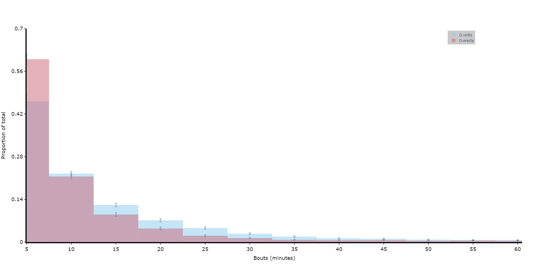
Find bouts of sleep
# If you haven't already analysed the dataset to find periods of sleep,0
# but you do have a column containing the movement as True/False.
# Call this method to find contiguous bouts of sleep according to a minimum length
new_df = df.sleep_contiguous(time_window_length = 60, min_time_immobile = 300) Sleep download functions as methods
# some of the download functions mentioned previously can be called as methods if the data wasn't previously analysed
# dont't call this method if your data was already analysed!
# If it's already analysed it will be missing columns needed for this method
new_df = df.motion_detector(time_window_length = 60)Visualising your data
Once the behavpy object is created, the print function will just show your data structure. If you want to see your data and the metadata at once, use the built in method .display()
# first load your data and create a behavpy instance of it
df.display()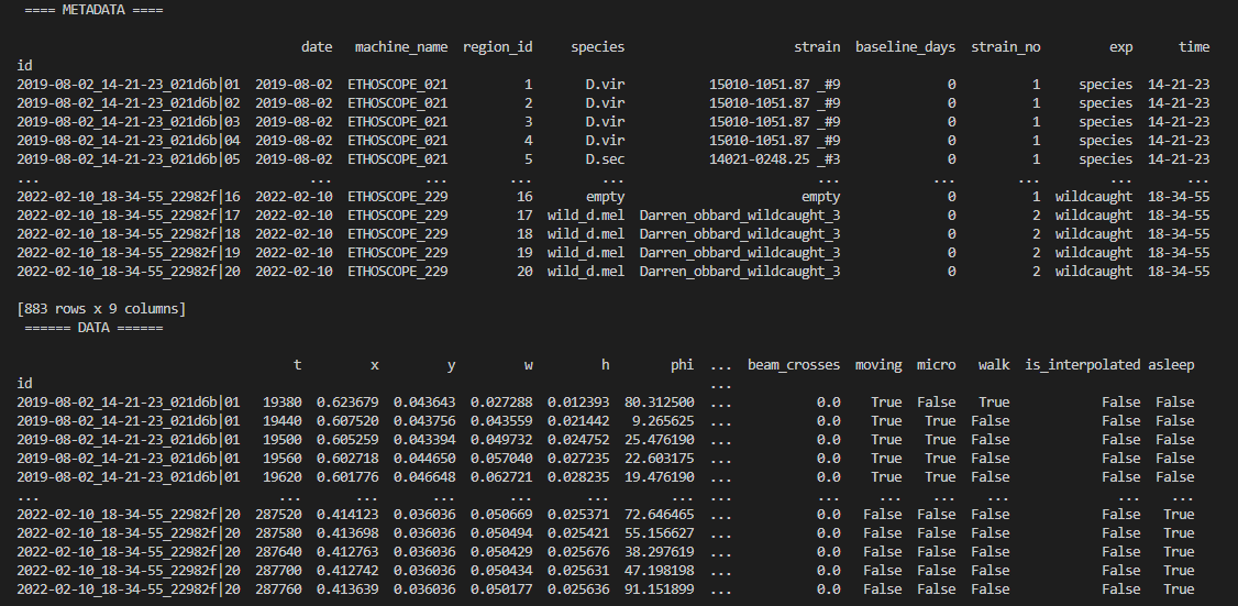
You can also get quick summary statistics of your dataset with .summary()
df.summary()
# an example output of df.summary()
output:
behavpy table with:
individuals 675
metavariable 9
variables 13
measurements 3370075
# add the argument detailed = True to get information per fly
df.summary(detailed = True)
output:
data_points time_range
id
2019-08-02_14-21-23_021d6b|01 5756 86400 -> 431940
2019-08-02_14-21-23_021d6b|02 5481 86400 -> 431940Be careful with the pandas method .groupby() as this will return a pandas object back and not a behavpy object. Most other common pandas actions will return a behavpy object.
Visualising your data
Whilst summary statistics are good for a basic overview, visualising the variable of interest over time is usually a lot more informative.
Heatmaps
The first port of call when looking at time series data is to create a heatmap to see if there are any obvious irregularities in your experiments.
# To create a heatmap all you need to write is one line of code!
# All plot methods will return the figure, the usual etiquette is to save the variable as fig
fig = df.heatmap('moving') # enter as a string which ever numerical variable you want plotted inside the brackets
# Then all you need to do is the below to generate the figure
fig.show()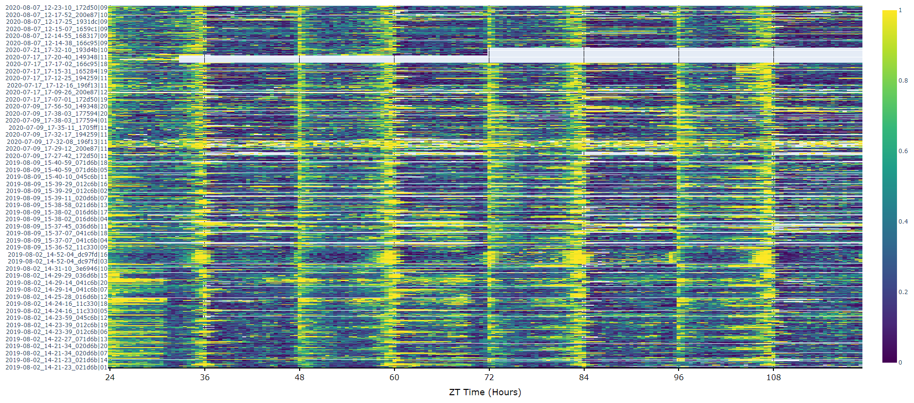
Plots over time
For an aggregate view of your variable of interest over time, use the .plot_overtime() method to visualise the mean variable over your given time frame or split it into sub groups using the information in your metadata.
# If wrapped is True each specimens data will be aggregated to one 24 day before being aggregated as a whole. If you want to view each day seperately, keep wrapped False.
# To achieve the smooth plot a moving average is applied, we found averaging over 30 minutes gave the best results
# So if you have your data in rows of 10 seconds you would want the avg_window to be 180 (the default)
# Here the data is rows of 60 seconds, so we only need 30
fig = df.plot_overtime(
variable = 'moving',
wrapped = True,
avg_window = 30
)
fig.show()
# the plots will show the mean with 95% confidence intervals in a lighter colour around the mean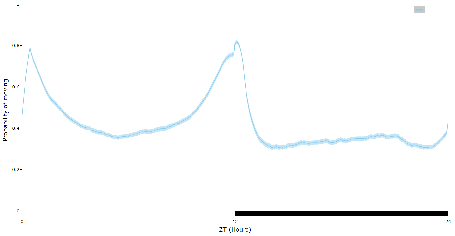
# You can seperate out your plots by your specimen labels in the metadata. Specify which column you want fromn the metadata with facet_col and then specify which groups you want with facet_args
# What you enter for facet_args must be in a list and be exactly what is in that column in the metadata
# Don't like the label names in the column, rename the graphing labels with the facet_labels parameter. This can only be done if you have a same length list for facet_arg. Also make sure they are the same order
fig = df.plot_overtime(
variable = 'moving',
facet_col = 'species',
facet_arg = ['D.vir', 'D.ere', 'D.wil', 'D.sec', 'D.yak'],
facet_labels = ['D.virilis', 'D.erecta', 'D.willistoni', 'D.sechellia', 'D.yakuba']
)
fig.show()
# if you're doing circadian experiments you can specify when night begins with the parameter circadian_night to change the phase bars at the bottom. E.g. circadian_night = 18 for lights off at ZT 18.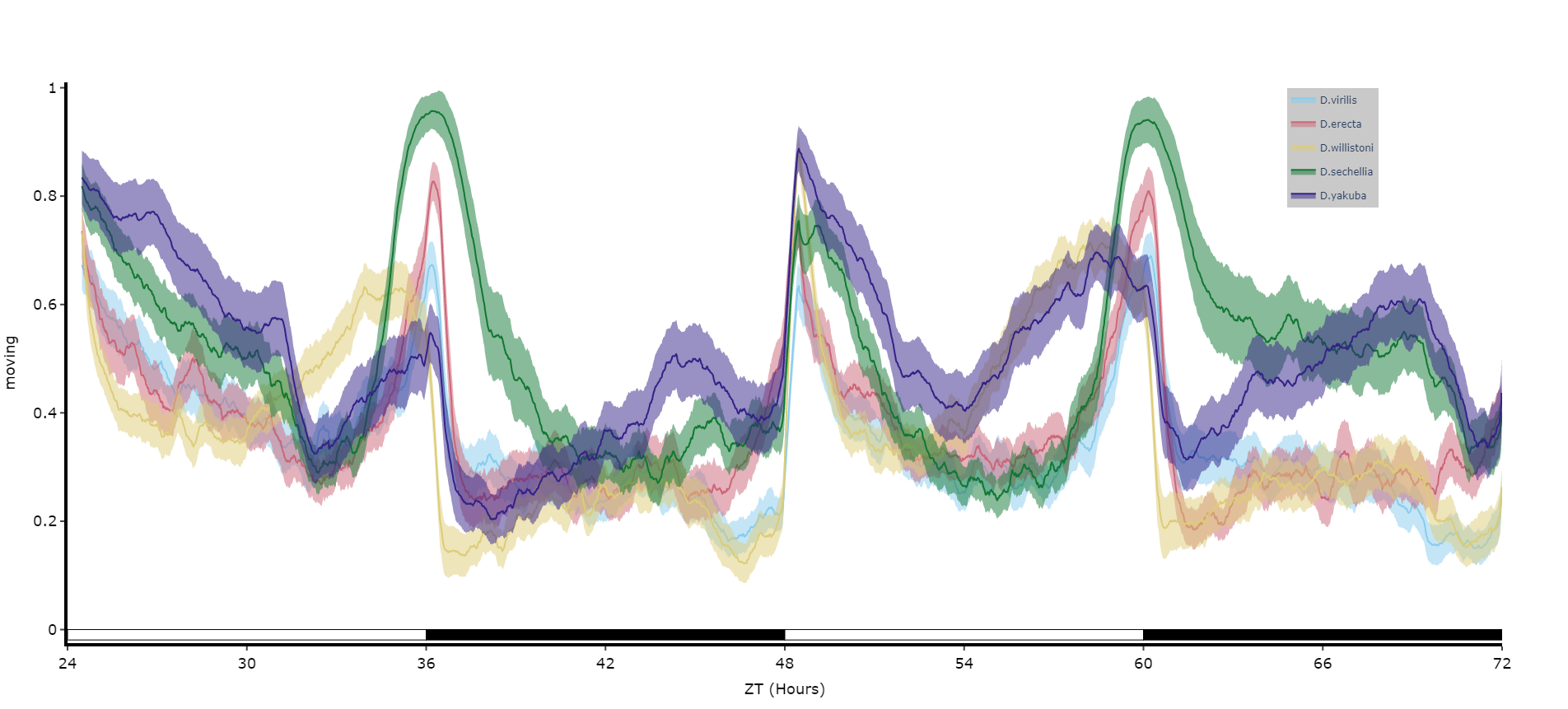
Quantifying sleep
The plots above look nice, but we often want to quantify the differences to prove what our eyes are telling us. The method .plot_quantify() plots the mean and 95% CI of the specimens to give a strong visual indication of group differences.
# Quantify parameters are near identical to .plot_overtime()
# For all plotting methods in behavpy we can add grid lines to better view the data and you can also add a title, see below for how
# All quantifying plots sill return two objects, the first will be the plotly figure as normal and the second a pandas dataframe with
# the calculated avergages per specimen for you to perform statistics on. You can do this via the common statistical package scipy or
# we recommend a new package DABEST, that produces non p-value related statisics and visualtion too.
# We'll be looking to add DABEST into our ecosytem soon too!
fig, stats_df = df.plot_quantify(
variable = 'moving',
facet_col = 'species',
facet_arg = ['D.vir', 'D.ere', 'D.wil', 'D.sec', 'D.yak']
title = 'This is a plot for quantifying',
grids = True
)
fig.show()
# Tip! You can have a facet_col argument and nothing for facet_args and the method will automatically plot all groups within that column. Careful though as the order/colour might not be preserved in similar but different plots
Performing Statistical tests
If you want to perform normal statistical tests then it's best to use Scipy, a very common python package for statistics with lots of online tutorial on how and when to use it. We'll run through a demonstration of one below. Below you'll see an example table of the data from the plot above.
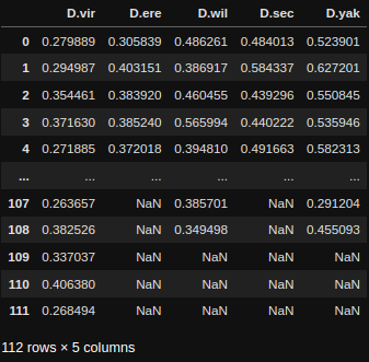
Given we don't know the distribution type of the data and that each group is independent we'll use a non-parametric group test, the Kruskal-Wallis H-test (the non-parametric version of a one-way ANOVA).
# First we need to import scipy stats
from scipy import stats
# Next we need the data for each specimen in a numpy array
# Here we iterate through the columns and send each column as a numpy array into a list
stat_list = []
for col in stats_df.columns.tolist():
stat_list.append(stats_df[col].to_numpy())
# Alternatively you can set each one as it's own variable
dv = stats_df['D.vir'].to_numpy()
de = stats_df['D.ere'].to_numpy()
... etc
# Now we call the Kruskal function, remember to always have the nan_policy set as 'omit' otherwise the output will be a NaN
# If using the first method (the * unpacks the list)
stats.kruskal(*stat_list, nan_policy = 'omit')
# If using the second
stats.kruskal(dv, de, ..., nan_policy = 'omit')
## output: KruskalResult(statistic=134.17956605297556, pvalue=4.970034343600611e-28)
# The pvalue ss below 0.05 so we can say that not all the groups have the same distribution
# Now we want to do some post hoc testing to find inter group significance
# For that we need another package scikit_posthocs
import scikit_posthocs as sp
p_values = sp.posthoc_dunn(stat_list, p_adjust = 'holm')
print(p_values)
## output: 1 2 3 4 5
1 1.000000e+00 2.467299e-01 0.000311 1.096731e-11 1.280937e-16
2 2.467299e-01 1.000000e+00 0.183924 1.779848e-05 7.958752e-08
3 3.106113e-04 1.839239e-01 1.000000 3.079278e-03 3.884385e-05
4 1.096731e-11 1.779848e-05 0.003079 1.000000e+00 4.063266e-01
5 1.280937e-16 7.958752e-08 0.000039 4.063266e-01 1.000000e+00
print(p_values > 0.05)
## output: 1 2 3 4 5
1 True True False False False
2 True True True False False
3 False True True False False
4 False False False True True
5 False False False True True
Quantify day and night
Often you'll want to compare a variable between the day and night, particularly total sleep. This variation of .plot_quantify() will plot the mean and 96% CI of a variable for a user defined day and night.
# Quantify parameters are near identical to .plot_quantify() with the addtion of day_length and lights_off which takes (in hours) how long the day is for the specimen (defaults 24) and at what point within that day the lights turn off (night, defaults 12)
fig, stats = df.plot_day_night(
variable = 'asleep',
facet_col = 'species',
facet_arg = ['D.vir', 'D.ere', 'D.wil', 'D.sec', 'D.yak'],
facet_labels = ['D.virilis', 'D.erecta', 'D.willistoni', 'D.sechellia', 'D.yakuba'],
day_length = 24,
lights_off = 12
)
fig.show()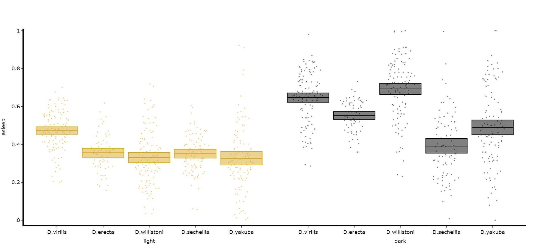
Compare variables
You may sometimes want to compare different but similar variables from your experiment, often comparing them across different experimental groups. Use .plot_compare_variables() to compare up to 24 different variables (we run out of colours after that...).
# Like the others it takes the regualar arguments. However, rather than the variable parameter it's variables, which takes a list of strings of the different columns you want to compare. The final variable in the list will have it's own y-axis on the right-hand side, so save this one for different scales.
# The most often use of this with the ethoscope data is to compare micro movements to walking movements to better understand the locomotion of the specimen, so lets look at that.
fig, stats = df.plot_compare_variables(
variables = ['mirco', 'walk']
facet_col = 'species',
facet_arg = ['D.vir', 'D.ere', 'D.wil', 'D.sec', 'D.yak'],
facet_labels = ['D.virilis', 'D.erecta', 'D.willistoni', 'D.sechellia', 'D.yakuba']
)
fig.show()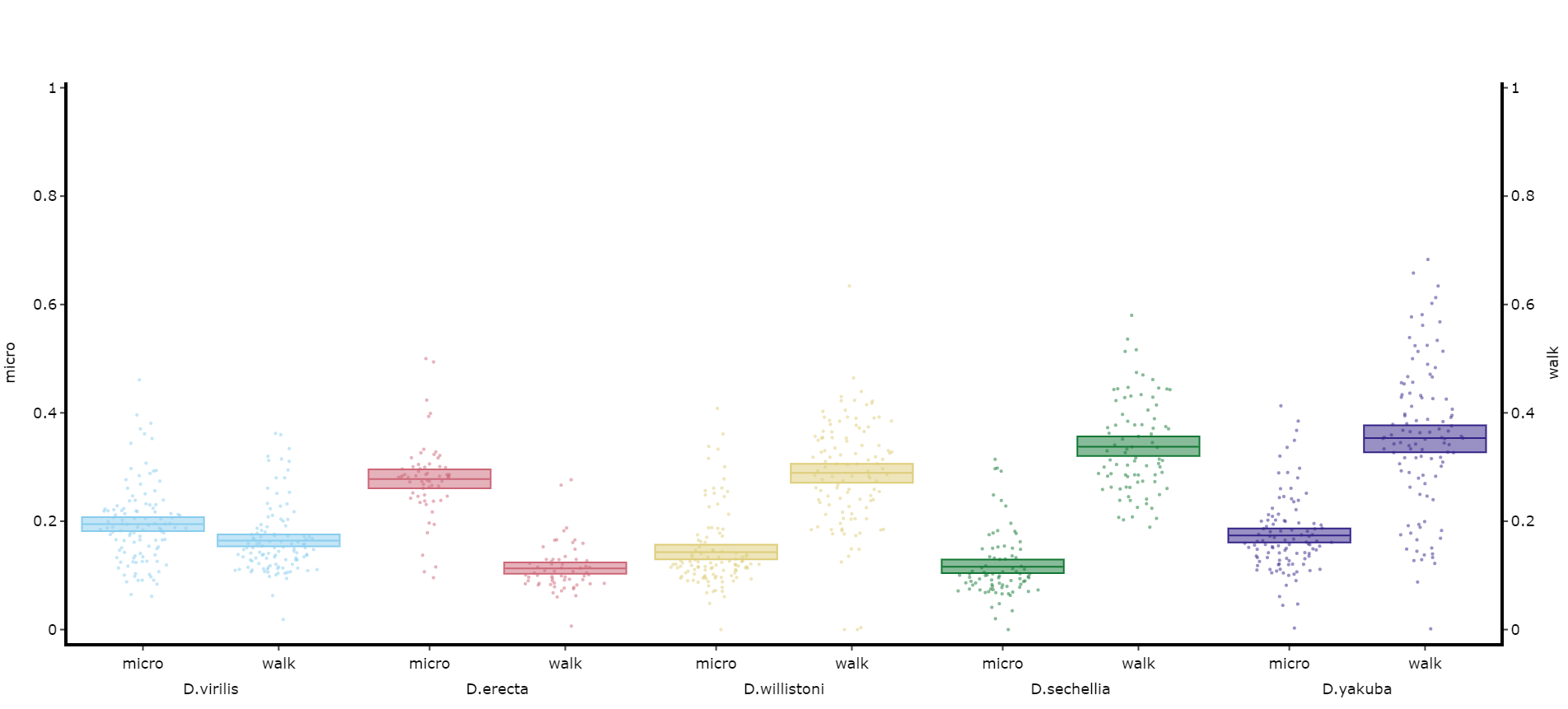
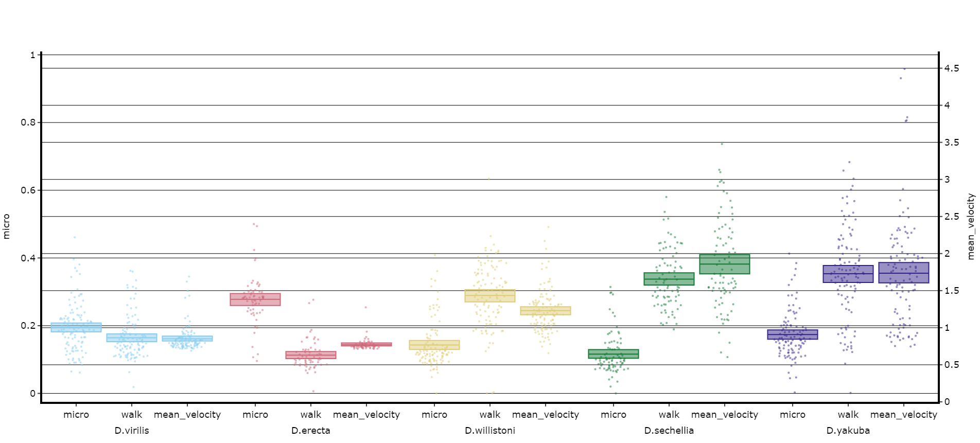
# Lets add the velocity of the specimen to see how it looks with different scales.
fig, stats = df.plot_compare_variables(
variables = ['mirco', 'walk', 'mean_velocity']
facet_col = 'species',
facet_arg = ['D.vir', 'D.ere', 'D.wil', 'D.sec', 'D.yak', 'D.sims'],
facet_labels = ['D.virilis', 'D.erecta', 'D.willistoni', 'D.sechellia', 'D.yakuba', 'D.Simulans'],
# Add grids to the plot so we can better see how the plots align
grids = True
)
fig.show()
Head to the Overview Tutorial for interactive examples of some of these plots. It also shows you how to edit the fig object after it's been generated if you wish to change things like axis titles and axis range.
Saving plots
As seen above all plot methods will produce a figure structure that you use .show() to generate the plot. To save these plots all we need to do is place the fig object inside a behavpy function called etho.save_figure()
You can save your plots as PDFs, SVGs, JPEGs or PNGS. It's recommended you save it as either a pdf or svg for the best quality and then the ability to alter then later.
You can also save the plot as a html file. Html files retain the interactive nature of the plotly plots. This comes in most useful when using jupyter notebooks and you want to see your plot full screen, rather than just plotted under the cell.
# simply have you returned fig as the argument alongside its save path and name to save
# remember to change the file type at the end of path as you want it
# you can set the width and height of the saved image with the parameters width and height (this has no effect for .html files)
etho.save_figure(fig, './tutorial_fig.pdf', width = 1500, height = 1000)
# or to get a better view of it and keep the interactability save it as a html file
etho.save_figure(fig, './tutorial_fig.html') # you can't change the height and width wehn saved as a htmlVisualising mAGO data
Within the Gilestro lab we have special adaptations to the ethoscope which includes the mAGO, a module that can sleep deprive flies manually and also deliver a puff of an odour of choice after periods of rest. See the documentation here: ethoscope_mAGO.
If you've performed a mAGO experiment then the data needs to be loaded in with the function puff_mago() which decides if a fly has responded if it's moved with the time limit post puff (default is 10 seconds).
Quantify response
The method .plot_response_quantify() will produce a plot of the mean response rate per group. Within the software for delivering a puff it can be set to have a random chance of occurring. I.e. if it's set to 50%, and the immobility criteria is met then the chance a puff will be delivered is 50/50. This gives us two sets of data, true response rate and the underlying likelihood a fly will just randomly move, which is called here Spontaneous Movement (Spon. Mov).
# The parameters other than response_col (which is the column of the response per puff) are the same as other quantify methods
fig, stats = df.plot_response_quantify(
resonse_col = 'has_responded',
facet_col = 'species',
)
fig.show()
Quantify response overtime
You can also view how the response rate changes over time with .plot_response_overtime(). For this method you'll need to load in the normal dataset, i.e. with motion_detector or sleep_annotation as the method needs to know at what point the puff occurred. The plot is per minute, so it's best to load it in with a time window of 60. If you have it higher the method won't work.
# Call the method on the normal behavpy table with the first argument the puff behavpy table
# The seconds argument decides if you're looking at runs of inactivty or activity,
# if you set the puff chance low enough you can probe activity too
fig, stats = df.plot_response_overtime(
response_df = puff_df,
activity = 'inactive',
facet_col = 'species'
)
fig.show()Behavpy - Circadian analysis
At the Gilestro lab we work on sleep and often need to do a lot of circadian analysis to compliment our sleep analysis. So we've got a dedicated suite of methods to analyse and plot circadian analysis. For the best run through of this please use the jupyter notebook tutorial that can be found at the end of this whole tutorial.
Circadian methods and plots
The below methods and plots should give a good insight into your specimens circadian rhythm. If you think another method should be added please don't hesitate to contact us and we'll see what we can do.
Head to the circadian notebook for an interactive run through of everything below.
Actograms
Actograms are one of the best initial methods to quickly visualise changes in the rhythm of a specimen over several days. An actogram double plots each days variable (usually movement) so you can compare each day with its previous and following day.
# .plot_actogram() can be used to plot indivdual specimens actograms or plot the average per group
# below we'll demonstrate a grouped example
fig = df.plot_actogram(
mov_variable = 'moving',
bin_window = 5, # the default is 5, but feel free to change it to smooth out the plot or vice versa
facet_col = 'period_group',
facet_arg = ['short', 'wt', 'long'],
title = 'Grouped Actogram')
fig.show()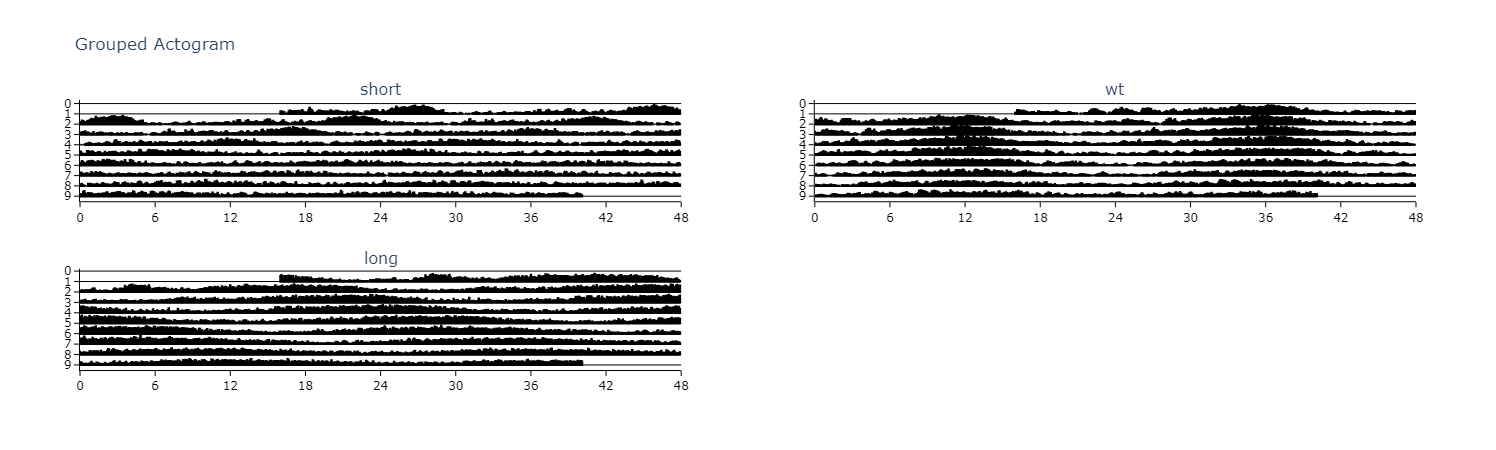
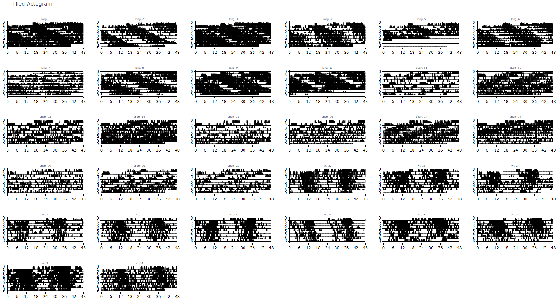
# plot_actogram_tile will plot every specimen in your behavpy dataframe
# Be careful if your dataframe has lots of flies as you'll get a very crowded plot!
fig = df.plot_actogram_tile(
mov_variable = 'moving',
labels = None, # By default labels is None and will use the ID column for the labels.
# However if individual labels in the metadata add that column here. See the tutorial for an example
title = 'Tiled Actogram')
fig.show()
Anticipation Score
Many animals including Drosophila have peaks of activity in the morning and evening as lights turn on and off respectively. Given this daily activity the activity score looks to quantify when the specimens internal clock anticipates these moments. The score is calculated as the ratio of the final 3 hours of activity prior to lights on and off compared to the whole 6 hours prior.
# Simply call the plot_anticipation_score() method to get a box plot of your results
# the day length and lights on/off time is 24 and 12 respectively, but these can be changed if you're augmenting the environment
fig, stats = df.plot_anticipation_score(
mov_variable = 'moving',
facet_col = 'period_group',
facet_arg = ['short', 'wt', 'long'],
day_length = 24,
lights_off = 12,
title = 'Anticipation Score')
fig.show()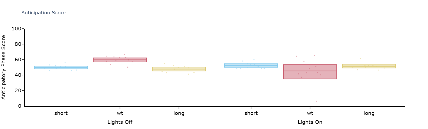
Periodograms
Initialising the Periodogram class
To access the methods that calculate and plot periodograms you need to initialise your data frame not as the base behavpy but as the periodogram behavpy class: etho.behavpy_periodogram()
per_df = etho.behavpy_periodogram(data, metadata, check = True)
# If you've already initialised it as a behavpy object
per_df = etho.behavpy_periodogram(df, df.meta, check = True)Calculating Periodograms
# The below method calculates the output from a periodogram function, returning a new dataframe with information about each period in your given range
# and the power for each period
# the periodogram can only compute 4 types of periodograms currently, choose from this list ['chi_squared', 'lomb_scargle', 'fourier', 'welch']
per_chi = per_df.periodogram(
mov_variable = 'moving',
periodogram = 'chi_squared', # change the argument here to the other periodogram types
period_range = [10,32], # the range in time (hours) we think the circadian frequency lies, [10,32] is the default
sampling_rate = 15, # the time in minutes you wish to smooth the data to. This method will interpolate missing results
alpha = 0.01 # the cutoff value for significance, i.e. 1% confidence
)
# Hint! Sometimes increasing the sampling_rate can improve you're periodograms. On average we found 15 to work best with our data, but it can be different for everyonePlotting Periodograms
Tile Plots
To get a good understanding of each individual specimen you can use the tiled periodogram plot
# Like the actogram_tile method we can rely on the ids of each specimen or we can use labels we created
fig = per_chi.plot_periodogram_tile(
labels = 'tile_labels',
find_peaks = True, # make find_peaks True to add a marker over significant peaks
title = 'Tiled Chi Squared Periodogram'
)
fig.show()
Grouped plots
Plot the average of each specimens periodograms to get a better view of the difference between experimental groups.
fig = per_chi.plot_periodogram(
facet_col = 'period_group',
facet_arg = ['short', 'wt', 'long'],
title = 'Grouped Chi Squared Periodogram'
)
fig.show() 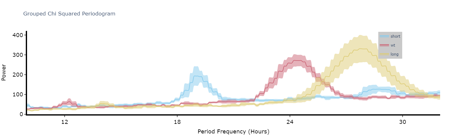
Quantifying plots
Like with the ethograms we can plot the above as quantification plot to see if what we see by eye is true statistically.
# Quantify the periodograms by finding the highest power peak and comparing it across specimens in a group
# call .quantify_periodogram() to get the results
fig, stats = per_chi.quantify_periodogram(
facet_col = 'period_group',
facet_arg = ['short', 'wt', 'long'],
title = 'Quantification of Chi Squared Periodogram'
)
fig.show()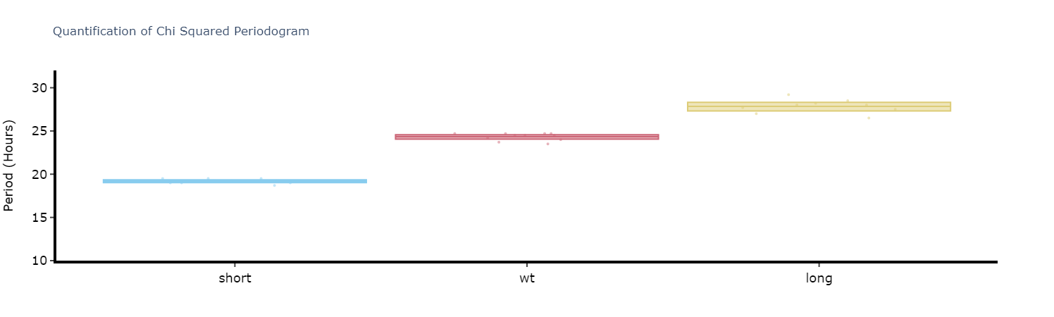
Wavelets
Wavelets are a special branch of periodograms as they are calculated in 3 dimensions rather than 2. Finding the period and power not for the whole given time, but rather broken down from the start to end. This then gives you an understanding of how rhythmicity changes over the course of your experiment, such as when you shift from LD to DD.
Wavelet plots are quite visually intensive, therefore the wavelet method will only compute and plot the average of all the data present in the data frame. Therefore, you will need to do some filtering beforehand to look at individual groups or an individual specimen.
# This method is powered bythe python package pywt, Head to https://pywavelets.readthedocs.io/en/latest/ for information about the pacakage and the other wavelet types
# filter your df prior to calling the plot
wt_df = per_df.xmv('period_group', 'wt')
fig = wt_df.wavelet(
mov_variable = 'moving',
sampling_rate = 15, # increasing the sampling rate will increase the resolution of lower frequencues (16-30 hours), but lose resolution of higher frequencies (2-8 hours)
scale = 156, # the defualt is 156, increasing this number will increase the resolution of lower frequencies (and lower the high frequencies), but it will take longer to compute
wavelet_type = 'morl', # the default wavelet type and the most commonly used in circadian analysis. Head to the website above for the other wavelet types or call the method .wavelet_types() to see their names
title = 'Wavelet: WT'
)
fig.show()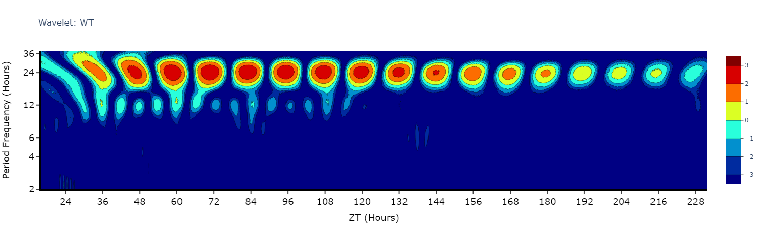
Behavpy - Hidden Markov Model
Behavpy_HMM is an extension of behavpy that revolves around the use of Hidden Markov Models (HMM) to segment and predict sleep and awake stages in Drosophila. This method is based on Wiggin et al PNAS 2020
Training an HMM
Behavpy_HMM is an extension of behavpy that revolves around the use of Hidden Markov Models (HMM) to segment and predict sleep and awake stages in Drosophila. A good introduction to HMMs is available here: https://web.stanford.edu/~jurafsky/slp3/A.pdf.
The provide a basic overview, HMMS are a generative probabilistic model, in which there is an assumption that a sequence of observable variables is generated by a sequence of internal hidden states. The transition probabilities between hidden states are assumed to follow the principles of a first order Markov chain.
Within this tutorial we will apply this framework to the analysis of sleep in Drosophila, using the observable variable movement to predict the hidden states: deep sleep, light sleep, quiet awake, active awake.
Hmmlearn
BehavpyHMM utilises the brilliant Python package Hmmlearn under the hood. Currently behavpy_HMM only uses the categorical version of the models available, as such it can only be trained and decode sequences that are categorical and in an integer form. If you wish to use their other models (multinomial, gaussian and guassian mixture models) or want to read more on their capabilities, head to their docs page for more information: https://hmmlearn.readthedocs.io/en/latest/index.html
Initialising behavpy_HMM
The HMM variant of behavpy is initialised in the same manner as the behavpy class. In fact, it is just a sub-classed version of behavpy so all the previous methods are still applicable, alongside the usual Pandas capabilities.
import ethoscopy as etho
# You can load you data using the previously mentioned functions
meta = etho.link_meta_index(meta_loc, remote, local)
data = etho.load_ethoscope(meta, min_time = 24, max_time = 48, reference_hour = 9.0)
# Remember you can save the data and metadata as pickle files, see the downloading section for a reminder about it
# to initialise a behavpy object, just call the class with the data and meta as arguments. Have check = True to ensure the ids match.
df = etho.behavpy_HMM(data, meta, check = True)Data curation
The data passed to the model needs to be good quality with long sequences containing minimal gaps and all a decent length in total.
Be careful when loading in your data. If you use the sleep_annotation() loading analysis function then it will automatically interpolate missing data as sleep giving you NaN (filler values) throughout your dataset. It's preferential to use the max_velocity_detector() function if you plan to use the HMM.
Use the .curate() and .bin_time() methods mentioned previously to curate the data. It is recommended to bin the data points to 60 second bins when analysing sleep and movement. But feel free to experiment with what works with your data.
import ethoscopy as etho
# load your data and metadata in and intialse your behavpy_HMM object
df = etho.behavpy_HMM(data, meta, check = True)
# it's often a good idea to filter out the start and beginning of experiments
df = df.t_filter(start_time = 24, end_time = 96)
# remove specimens with less than a days worth of data (if binned to 60 seconds)
df = df.curate(points = 1440)
# Any NaN values will throw an error when trying to train the HMM. It's good practice to check the data for any
# If below returns True you have NaN values in your data
print(np.any(np.isnan(df['YOUR COLUMN'].to_numpy())))
# If it is True then look at those values and replace or remove (the whole specimen) from the dataset
# Use below to view which rows have NaNs, see pandas documnetation for more information on how to replace NaN values
df[df['YOUR COLUMN'].isnull()]
# binning the variable can be done within the .hmm_train() method, see next!Training a HMM
Behavpy_HMM provides a wrapper function for hmmlearn multinomial model. The method extends the hmmlearn model by automatically manipulating the data into a readable format for training. Additionally, the method provides the option to randomise the initialised transmission / observable parameters to train the model several times. Each iterative model is compared to the best previous performing model with the hopes of avoiding reach a local minima during hmmlearns own internal iterative process.
As mentioned previously the HMM used here is categorical, therefore only select data that is categorically discrete. For example here we will be using activity, with not moving being one state and moving the other. These states as data must be in integer form. So this example, not moving will = 0 and moving will = 1. Follow this example if using more states, so if you have three states use the integers 0, 1, 2.
In setting up the HMM you have to specify how many hidden states your system will have and the what states can transition into one another. See below for an example.
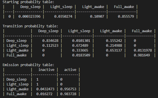
Setting up
# the setup for .hmm_train()
# name your hidden states and observables. This is just purely for visualising the output and setting the number of hidden states!
hidden_states = ['Deep sleep', 'Light sleep', 'Light awake', 'Active awake']
observable_variables = ['inactive', 'active']
# if you believe your hidden states can only transition into specific states or there's a flow you can setup the model to train with this in mind. Have the transitions you want to happen set as 'rand' and those that can't as 0
t_prob = np.array([['rand', 'rand', 'rand', 0.00],
['rand', 'rand', 'rand', 0.00],
[0.00, 'rand', 'rand', 'rand'],
[0.00, 'rand', 'rand', 'rand']])
# Make sure your emission matrix aligns with your categories
em_prob = np.array([[1, 0],
[1,0],
['rand', 'rand'],
['rand', 'rand']])
# the shape of each array should be len(hidden_states) X len(names). E.g. 4x4 and 4x2 respectivelyYou can leave trans_probs and em_prob as None to have all transitions randomised before each iteration
Training
# add the above variables to the hmm_train method
# iterations is the number of loops with a new randomised parameters
# hmm_interactions is the number of loops within hmmlearn before it stops. This is superceeded by tol, with is the difference in the logliklihood score per interation within hmmlearn
# save the best performing model as a .pkl file
df.hmm_train(
states = hidden_states,
observables = observable_variables,
var_column = 'moving',
trans_probs = t_prob,
emiss_probs = em_prob,
start_probs = None,
iterations = 10,
hmm_iterations = 100,
tol = 2,
t_column = 't',
bin_time = 60,
file_name = 'experiment_hmm.pkl', # replace with your own file name
verbose = False)
# If verbose is true the logliklihood per hmm iteraition is printed to screenDiving deeper! To find the best model the dataset will be split into a test (10%) and train (90%) datasets. Each successive model will be scored against the best on the test dataset. The best scoring model will be the final save to your file name.
Visualising with the HMM
The best way to get to grips with your newly trained HMM is to decode some data and has a look at it visually.
Single plots
# Like plot_overtime() this method will take a single variable and trained hmm, and plot them over time.
# If you're using behavpy_HMM to look at sleep using the 4 state structure you don't have to specify labels and colours, as they are pre written. However, if you aren't please specify.
# use below to open your saved trained hmmlearn object
with open('/Users/trained_hmms/4_states_hmm.pkl', 'rb') as file:
h = pickle.load(file)
fig = df.plot_hmm_overtime(
hmm = h,
variable = 'moving',
labels = ['Deep sleep', 'Light sleep', 'Light awake', 'Full awake'],
# colours = ['blue', 'green', 'yellow', 'red'], # example colours
wrapped = True,
bin = 60
)
fig.show()
# You cannot facet using this method, see the next plot for faceting 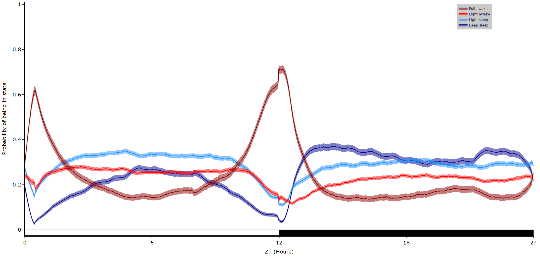
Faceted plots
To reduce clutter when faceting the plot will become a group of subplots, with each subplot the collective plots of each specimen for each hidden state.
# plot_hmm_split works just like above, however you need to specify the column to facet by. You can also specify the arguments if you don't want all the groups from the facet column
fig = df.plot_hmm_split(
hmm = h,
variable = 'moving',
facet_col = 'species',
wrapped = True,
bin = 60
)
fig.show()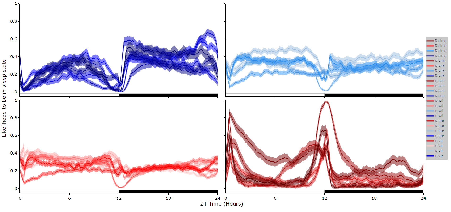
# You don't always want to decode every group with the same hmm. In fact with different species, mutants,
# subgroups you should be training a fresh hmm
# if you pass a list to the hmm parameter the same length as the
# facet_arg argument the method will apply the right hmm to each group
fig = df.plot_hmm_split(
hmm = [hv, he, hw, hs, hy],
variable = 'moving',
facet_labels = ['D.virilis', 'D.erecta', 'D.willistoni', 'D.sechellia', 'D.yakuba']
facet_col = 'species',
facet_arg = ['D.vir', 'D.ere', 'D.wil', 'D.sec', 'D.yak'],
wrapped = True,
bin = [60, 60, 60, 60, 60]
)
fig.show()
Quantify time in each state
# Like plot_quantify() this method will quantify how much of the time each specimen is within each state.
fig, stats = df.plot_hmm_quantify(
hmm = [hv, he, hw, hs, hy],
variable = 'moving',
facet_labels = ['D.virilis', 'D.erecta', 'D.willistoni', 'D.sechellia', 'D.yakuba']
facet_col = 'species',
facet_arg = ['D.vir', 'D.ere', 'D.wil', 'D.sec', 'D.yak'],
bin = [60, 60, 60, 60, 60]
)
fig.show()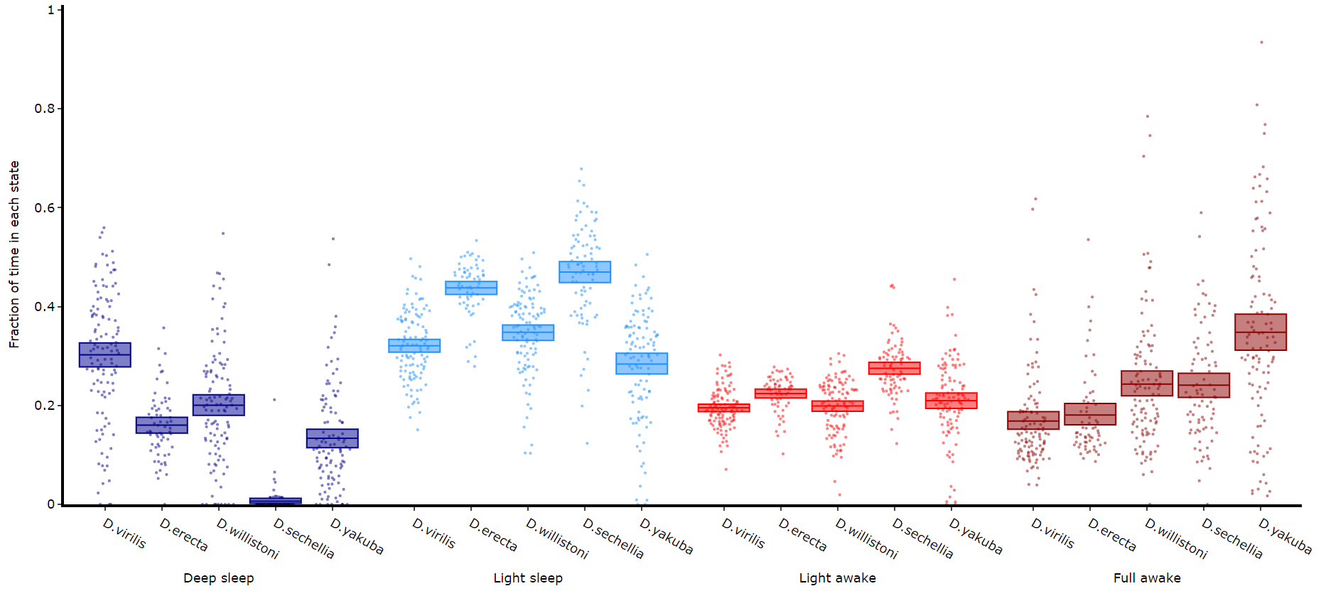
Quantifying length of each state
Its a good idea to look at the length of each state to gain an understanding of how the model is separating your data. There are two length methods 1) one to plot the mean lengths per state per specimen and 2) a plot to show the maximum and minimum state length per group.
# all hmm quantifying plots have the same parameters, so just change the method name and you're good to go
fig, stats = df.plot_hmm_quantify_length(
hmm = [hv, he, hw, hs, hy],
variable = 'moving',
facet_labels = ['D.virilis', 'D.erecta', 'D.willistoni', 'D.sechellia', 'D.yakuba']
facet_col = 'species',
facet_arg = ['D.vir', 'D.ere', 'D.wil', 'D.sec', 'D.yak'],
bin = [60, 60, 60, 60, 60]
)
fig.show()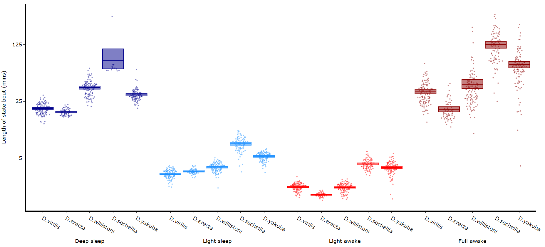
# The length min/max method only shows the the min and maximum points as a box
# this plot doesnt return any stats, as it is just the min/max and mean values
fig = df.plot_hmm_quantify_length_min_max(
hmm = [hv, he, hw, hs, hy],
variable = 'moving',
facet_labels = ['D.virilis', 'D.erecta', 'D.willistoni', 'D.sechellia', 'D.yakuba']
facet_col = 'species',
facet_arg = ['D.vir', 'D.ere', 'D.wil', 'D.sec', 'D.yak'],
bin = [60, 60, 60, 60, 60]
)
fig.show()
# Below you can see when the model seperates light sleep from deep sleep 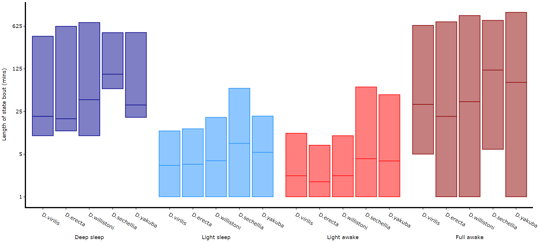
Quantifying transitions
The time in each state and the average length are good overview stats, but can be misleading about how often a state occurs if the state is short. This next method quantifies the amount of times a state is transitioned into, effectively counting the instances of the state regardless of time.
fig, stats = df.plot_hmm_quantify_transition(
hmm = [hv, he, hw, hs, hy],
variable = 'moving',
facet_labels = ['D.virilis', 'D.erecta', 'D.willistoni', 'D.sechellia', 'D.yakuba']
facet_col = 'species',
facet_arg = ['D.vir', 'D.ere', 'D.wil', 'D.sec', 'D.yak'],
bin = [60, 60, 60, 60, 60]
)
fig.show()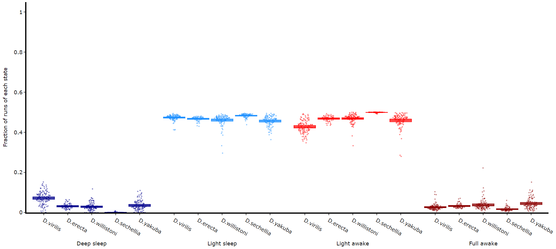
Raw decoded plot
Sometimes you will want to view the raw decoded plots of individual specimens to get a sense of the daily ebb and flow. .plot_hmm_raw() will plot 1 or more individual specimens decoded sequences.
# The ID of each specimen will be printed to the screen in case you want o investigate one or som further
fig = df.plot_hmm_raw(
hmm = h,
variable = 'moving',
num_plots = 5, # the number of different specimens you want in the plot
bin = 60,
title = ''
)
fig.show()
# Addtionally, if you have response data from mAGO experiments you can add that behavpy dataframe to
# highlight points of interaction and their response
# Purple = response, lime = no response
## df.plot_hmm_raw(mago_df = mdf, hmm = h, variable = 'moving', num_plots = 5, bin = 60, title = '', save = False)Jupyter tutorials
Ethoscopy is best used in a Jupyter instance. We provide a pre-baked docker container that comes with multiuser JupyterHub and the ethoscopy package: ethoscope-lab. Ethoscope-lab runs the Python 3.8 Kernel and the R Kernel and features an installation of rethomics too.
One of the biggest advantages of using Jupyter Notebook is that data treatment can be shared publicly in the most readable format. This is a great tool to aid scientific reproducibility and transparency to your publications.
We provide here below several example notebooks.
- Overview tutorial notebook (here)
- HMM tutorial notebook (here)
- Circadian tutorial notebook (here)
- Navigating databases (here)
- Converting data to HCTSA format (here)
Tutorial 1 — Overview: working with ethoscope data
Auto-generated from
tutorial_notebook/1_Overview_tutorial.ipynb. Executed against the seaborn canvas so every figure is inline as a static PNG. Plotly-only cells are kept for context and marked as placeholders — for the interactive version, run the source notebook.
Tutorial number 1
Working with ethoscope data
The tutorial will guide you through loading data, visualisation and plotting using the common sleep functions
1. Load the dummy dataset
import ethoscopy as etho
import pandas as pd
# This tutorial requires version 2.0.5 or greater
etho.__version__
'2.0.5'
One-time setup: fetch the tutorial datasets
The tutorial pickle files (~36 MB total, dominated by overview_data.pkl) are not bundled with the PyPI package, to keep pip install ethoscopy lean. Users of the ethoscope-lab Docker image can skip this cell — the pickles are already baked into the image.
Run the cell below once per environment to download them into ~/.cache/ethoscopy/tutorial_data/. Subsequent runs are idempotent.
# Idempotent: skips files that are already present.
import ethoscopy as etho
etho.download_tutorial_data()
Tutorial data downloaded into the user cache.
# import this function to get the tutorial dataset
from ethoscopy.misc.get_tutorials import get_tutorial
# There's some dummy data within ethoscopy for you to play with — use the function below with the argument 'overview'
# to get the data and metadata that will work with this notebook.
data, metadata = get_tutorial('overview')
# Create the behavpy object, combining your data and metadata into a linked dataframe.
# `check=True` removes metadata columns that are no longer needed post-download.
# `canvas` selects the plotting backend: 'plotly' (interactive) or 'seaborn' (static).
# For this static render we use seaborn throughout; set canvas='plotly' locally if you want the interactive version.
df = etho.behavpy(data, metadata, palette='Set2', check=True, canvas='seaborn')
dfp = etho.behavpy(data, metadata, palette='Set2', check=True, canvas='plotly')
df.canvas
'seaborn'
# Save as a pickle so subsequent sessions can skip the linking step.
df.to_pickle('./tutorial_dataframe.pkl')
# Load back with pandas — `df` is a behavpy subclass of DataFrame so pickling round-trips natively.
df = pd.read_pickle('./tutorial_dataframe.pkl')
# Display an excerpt of both metadata and data together
df.display()
(Metadata table: 39 specimens × 7 columns, Data table: 327031 rows × 16 columns. Full listing elided in the docs — run the notebook locally to view.)
# Or just the metadata
df.meta
| id | date | machine_name | region_id | sex | sleep_deprived | exp_group | time |
|---|---|---|---|---|---|---|---|
| 2016-04-04_17-39-22_033aee|01 | 2016-04-04 | ETHOSCOPE_033 | 1 | M | True | 1 | 17-39-22 |
| 2016-04-04_17-39-22_033aee|02 | 2016-04-04 | ETHOSCOPE_033 | 2 | M | False | 1 | 17-39-22 |
| … (39 specimens total — 20 from ETHOSCOPE_033, 19 from ETHOSCOPE_009) |
# Summary statistics of the whole experiment
df.summary()
behavpy table with:
individuals 39
metavariable 7
variables 16
measurements 327031
# Detailed per-specimen data points / time range
df.summary(detailed=True)
(Detailed per-specimen table — each individual has ~9600 data points spanning t = 31140 → 608340. Elided in the docs.)
2. Curate the data
# Heatmaps give a quick overview and make dead/abnormal specimens obvious.
fig = df.heatmap(variable='asleep');

# Remove specimens that stopped moving for an extended period ("dead").
# Data before their death is retained.
df = df.curate_dead_animals()
# Filter by time — cut the fragmentary first half-day and anything after the experimental window.
df = df.t_filter(start_time=24, end_time=144)
# Re-heatmap to see the effect
fig = df.heatmap(variable='asleep')

# Sleep-deprived subgroup
fig = df.xmv('sleep_deprived', True).heatmap(variable='asleep', title='Sleep Deprived Flies')

# Non-sleep-deprived subgroup
fig = df.xmv('sleep_deprived', False).heatmap(variable='asleep', title='Non-Sleep Deprived Flies')

# There's still one specimen in the control group that looks abnormal — almost always asleep,
# but not caught by curate_dead_animals(). Remove it explicitly after zooming in to get its id.
df = df.remove('id', '2016-04-04_17-39-05_009aee|02')
fig = df.heatmap(variable='asleep')

3. Visualise and save the sleep data
# Ethogram of the whole dataset — solid line = mean, shaded area = 95% CI.
fig = df.plot_overtime(variable='asleep', title='Whole Dataset Ethogram')

# Wrapped over a day to emphasise the circadian structure.
fig = df.plot_overtime(variable='asleep', wrapped=True, title='Ethogram — wrapped daily')

# Split by experimental group.
fig = df.plot_overtime(variable='asleep', facet_col='exp_group', title='Ethogram by experimental group')

# Focus on the rebound window and relabel the legend.
zoomin_df = df.t_filter(start_time=72, end_time=132)
fig = zoomin_df.plot_overtime(
variable='asleep',
facet_col='sleep_deprived', facet_arg=[True, False],
facet_labels=['Sleep Deprived', 'Control'],
title='Sleep deprived vs control',
)

# Plotly-only: make_tile arranges multiple overtime plots in subplots.
from functools import partial
fig_fun = partial(
dfp.plot_overtime, variable='asleep',
facet_col='sleep_deprived', facet_arg=[True, False],
facet_labels=['Sleep Deprived', 'Control'],
)
fig = dfp.make_tile(facet_tile='exp_group', plot_fun=fig_fun)
fig.show()
(Plotly figure — run the notebook locally for the interactive version.)
# Additional plot_overtime parameters: smoothing window, custom day_length / lights_off, gridlines, and a custom colour list.
fig = df.plot_overtime(
variable='asleep',
facet_col='sleep_deprived', facet_arg=[True, False],
facet_labels=['SD', 'Non SD'],
title='Whole Dataset Ethogram with tweaks',
avg_window=60, day_length=30, lights_off=15, grids=True,
col_list=['#0eeebe', '#d824db'],
)

# Same plot, but Plotly — deselect legend items in the browser to declutter.
fig = dfp.plot_overtime(
variable='asleep',
facet_col='sleep_deprived', facet_arg=[True, False],
facet_labels=['SD', 'Non SD'],
title='Whole Dataset Ethogram — Plotly',
avg_window=60, day_length=30, lights_off=15, grids=True,
col_list=['#0eeebe', '#d824db'],
)
fig.show()
(Plotly figure — run the notebook locally for the interactive version.)
# Saving figures: HTML (keeps Plotly interactivity), PDF or PNG (static, any canvas).
fig = df.plot_overtime(variable='asleep', facet_col='exp_group')
df.save_figure(fig, './tutorial_plot.pdf', width=1500, height=1500)
df.save_figure(fig, './tutorial_plot.png', width=2000, height=1500)
Saved to ./tutorial_plot.pdf
Saved to ./tutorial_plot.png

# plot_quantify — returns (fig, stats_df). Useful both for the figure and for the raw per-specimen values.
temp_df = df.t_filter(start_time=24, end_time=96)
fig, stats_quant = temp_df.plot_quantify(
variable='asleep',
facet_col='sleep_deprived', facet_arg=[True, False],
facet_labels=['Sleep Deprived', 'Control'],
title='Quantification of baseline sleep',
)

# The returned stats dataframe carries the per-specimen means and group label,
# ready for downstream statistical analysis.
stats_quant.head()
| id | asleep_mean | asleep_std | sleep_deprived |
|---|---|---|---|
| 2016-04-04_17-39-22_033aee|11 | 0.306 | 0.461 | Control |
| 2016-04-04_17-39-22_033aee|19 | 0.326 | 0.469 | Control |
| 2016-04-04_17-39-22_033aee|08 | 0.403 | 0.491 | Control |
| 2016-04-04_17-39-05_009aee|19 | 0.421 | 0.494 | Control |
| 2016-04-04_17-39-05_009aee|17 | 0.400 | 0.490 | Control |
| … |
4. Quantify and compare
# Rebound sleep — 3-hour window after the deprivation ends.
temp_df = df.t_filter(start_time=120, end_time=123)
fig, stats_deprivation = temp_df.plot_quantify(
variable='asleep',
facet_col='sleep_deprived', facet_arg=[True, False],
facet_labels=['Sleep Deprived', 'Control'],
title='Quantification of rebound sleep',
)

# Plotly version applies z-score filtering (>3 std removed) by default.
temp_df = dfp.t_filter(start_time=120, end_time=123)
fig, stats_deprivation = temp_df.plot_quantify(
variable='asleep',
facet_col='sleep_deprived', facet_arg=[True, False],
facet_labels=['Sleep Deprived', 'Control'],
z_score=True,
title='Quantification of rebound sleep',
)
fig.show()
(Plotly figure — run the notebook locally for the interactive version.)
# Day / night split for the same window.
temp_df = df.t_filter(start_time=96, end_time=120)
fig, stats_day_night = temp_df.plot_day_night(
variable='asleep',
facet_col='sleep_deprived', facet_labels=['ctrl', 'SD'],
title='Quantification of day and night',
)

# plot_compare_variables — two-y-axis plot comparing multiple variables. Plotly-only.
temp_df = dfp.t_filter(start_time=24, end_time=96)
fig, stats_multiple = temp_df.plot_compare_variables(
variables=['micro', 'walk', 'max_velocity'],
facet_col='sleep_deprived', facet_arg=[True, False],
facet_labels=['Sleep Deprived', 'Control'],
title='Micromovements vs walking',
)
fig.show()
(Plotly figure — run the notebook locally for the interactive version.)
5. Editing the figure object before display
The fig returned by every plotting method is the native matplotlib/Axes (seaborn canvas) or Plotly figure object, so you can tweak anything before showing or saving.
# Seaborn canvas — matplotlib API.
plotter = df
fig = plotter.plot_overtime(variable='asleep', facet_col='exp_group')
fig.axes[0].set_xlabel('new x-axis label', color='red', fontsize=30)
fig.axes[0].set_ylabel('new y-axis label', color='blue', fontsize=30)

# Change y-axis range and tick positions.
import numpy as np
plotter = df
fig = plotter.plot_overtime(variable='asleep', facet_col='exp_group')
fig.axes[0].set_ylim([0, 2])
fig.axes[0].yaxis.set_ticks(np.arange(0, 2.1, 0.5))

6. Exporting the notebook for publications
Notebooks double as a record of the analysis. Export this entire notebook as HTML to share code + figures without a Python install on the reader's side:
File → Save and Export Notebook As → HTML
Or, if you want a static version that lives alongside the documentation, the same nbconvert --execute --to markdown pipeline used to generate this page does the job.
Tutorial 2 — HMM: hidden behavioural states
Auto-generated from
tutorial_notebook/2_HMM_tutorial.ipynb. Executed against the seaborn canvas so every figure is inline as a static PNG. Plotly-only cells are kept for context and marked as placeholders — for the interactive version, run the source notebook.
Ethoscopy - HMM tutorial
This tutorial assumes you have some basic knowledge of Ethoscopy, if you don't please head to the overview tutorial first.
For this tutorial we will be training a Hidden Markov Model (HMM) using an ethoscopy wrapper class for the python package Hmmlearn, see https://hmmlearn.readthedocs.io/en/latest/ for more details on what this excellent package can do. A good introduction to HMM's is available here: https://web.stanford.edu/~jurafsky/slp3/A.pdf
Ethoscopy adapts their Categorical HMM, as such the model can only be trained using discrete data represented as integers starting with 0 as the first. I.e. "Cat 1 = 0, Cat 2 = 1, ..."
At the Gilestro lab we train our model using movement data from the Ethoscope system, using tested parameter limits for velocity as movement we categorise movement as either True or False, or 1 or 0. During the setup we found data binned to 60 seconds (1 min) and then trained best recapitulated the sleep of CS drosophila.
1. Load the dummy dataset
import pickle
import ethoscopy as etho
import numpy as np
# This tutorial required version 1.1.8 or greater
etho.__version__
'2.0.5'
One-time setup: fetch the tutorial datasets
The tutorial pickle files (~36 MB total, dominated by overview_data.pkl) are not bundled with the PyPI package, to keep pip install ethoscopy lean.
Run the cell below once per environment to download them into the installed package directory. Subsequent runs are idempotent (already-present files are skipped).
You can also fetch them manually from https://github.com/gilestrolab/ethoscopy/tree/main/src/ethoscopy/misc/tutorial_data.
# Idempotent: skips files that are already present.
import ethoscopy as etho
etho.download_tutorial_data()
[skip] overview_data.pkl (already present)
[skip] overview_meta.pkl (already present)
[skip] circadian_data.pkl (already present)
[skip] circadian_meta.pkl (already present)
[skip] 4_states_F_WT.pkl (already present)
[skip] 4_states_M_WT.pkl (already present)
Tutorial data ready in: /home/gg/.cache/ethoscopy/tutorial_data
PosixPath('/home/gg/.cache/ethoscopy/tutorial_data')
# import this function to get the tutorial dataset
from ethoscopy.misc.get_tutorials import get_tutorial
# We'll be using the same dataset as in the overview tutorial, so use the same function below with the argument 'overview'
# Load the data and metadata, and then intialise it into a behavpy_HMM
data, metadata = get_tutorial('overview')
df = etho.behavpy(data, metadata, canvas = 'seaborn', check = True)
dfp = etho.behavpy(data, metadata, canvas = 'plotly', check = True)
2. Curate the Data
# First we'll call the method to remove dead specimens
# df = df.curate_dead_animals()
# We'll also remove the specimen we noticed in the overview tutorial that was missed by the above method
df = df.remove('id', '2016-04-04_17-39-05_009aee|02')
# As we saw in the overview tutorial the dataset has half the specimens sleep deprived later in the experiment
fig = df.heatmap(variable = 'asleep')
fig.show()
/home/gg/Code/ethoscope_project/ethoscopy/src/ethoscopy/behavpy_core.py:1605: FutureWarning: DataFrameGroupBy.apply operated on the grouping columns. This behavior is deprecated, and in a future version of pandas the grouping columns will be excluded from the operation. Either pass `include_groups=False` to exclude the groupings or explicitly select the grouping columns after groupby to silence this warning.
tdf.groupby("id", group_keys=False).apply(
/tmp/ipykernel_554230/4143008177.py:3: UserWarning: FigureCanvasAgg is non-interactive, and thus cannot be shown
fig.show()

# When training a HMM you want a specimens basline data as normal conditions, so for this excerise we'll want to trim the dataset
# We can see from the heatmap that the sleep deprivation begins at 108 hours (ZT 12), we'll also trim the first day data as the specimens settle in
df = df.t_filter(start_time = 24, end_time = 108)
# It's also key to have as few missing values as possible when training the data, as the model assumes a consitent time gap between each point
# Our dataset now has 3.5 days with time bins of 60 seconds, so if a specimen was to have maximum data points for that time they would have
# (86400/60) * 3.5 rows of data. Lets not take any chances and only take specimens with that exact amount
df = df.curate(points = (86400/60) * 3.5)
# If any of the data passed to the model to be trained contains NaN values it will throw an error
# So lets check our data for NaN values
df['moving'][df['moving'].isnull()]
id
2016-04-04_17-39-22_033aee|01 NaN
Name: moving, dtype: object
# We have one NaN value, which is enough to crash the whole thing!
# Luckily pandas has built in methods to replace NaN values, use ffill() (from the row above) for forward fill NaNs or bffill() to back fill (from the row below).
# Lets to see if it worked
df['moving'][df['moving'].isnull()]
id
2016-04-04_17-39-22_033aee|01 NaN
Name: moving, dtype: object
3. Setup
# Now we're setup we can call the training method
# iterations is the number of times you want to iterate and train starting with new transiton and emission probabilities. It's recommended to have this higher than 3
# but for the tutorial we'll keep it low for the sake of time. More iterations mean you're more likely to find the best fitting model and
# hmm_iterations is the number of times the HMM will iterate with newer parameters before stopping
# tol is the the value for the difference in log liklihood after each iteration, once the value equals your input the model will stop updating the parameters
# After each time the transiton and emission probabilities are randomised and a model is produced, a score of logliklihood will be generated against 10% of the data,
# each new model will be scored against this and the best one will be returned at the end. Change the size of the test batch with test_size
# Save the best model to your local as a pickle file with file_name. The method will also return the trained model, but it's best to save it to a file
h = df.hmm_train(
states = hidden_states,
observables = observables,
var_column = 'moving',
trans_probs = t_prob,
emiss_probs = em_prob,
start_probs = None,
iterations = 3,
hmm_iterations = 100,
tol = 2,
t_column = 't',
bin_time = 60,
test_size = 10,
file_name = 'tutorial_hmm.pkl', # replace with your own file name. If you already have a pickle file named this, it will test the first iteration against it.
verbose = False)
# If verbose is True it will print to screen the logliklihood score of each hmm iteration
Iteration 1 of 3
True Convergence:True
Final log liklihood score:-71355.25073897192
Iteration 2 of 3
True Convergence:True
Final log liklihood score:-71387.66974287847
Iteration 3 of 3
True Convergence:True
Final log liklihood score:-71382.64987334394
Starting probabilty table:
| | Deep sleep | Light sleep | Light awake | Active awake |
|----|--------------|---------------|---------------|----------------|
| 0 | 0 | 0 | 0.25689 | 0.74311 |
Transition probabilty table:
| | Deep sleep | Light sleep | Light awake | Active awake |
|--------------|--------------|---------------|---------------|----------------|
| Deep sleep | 0.154846 | 0.481724 | 0.363429 | 0 |
| Light sleep | 0.602652 | 0.337834 | 0.0595133 | 0 |
| Light awake | 0 | 0.243226 | 0.744384 | 0.0123892 |
| Active awake | 0 | 0 | 0.0165169 | 0.983483 |
Emission probabilty table:
| | Inactive | Active |
|--------------|------------|----------|
| Deep sleep | 1 | 0 |
| Light sleep | 1 | 0 |
| Light awake | 0.175193 | 0.824807 |
| Active awake | 0.0207276 | 0.979272 |
# if .hmm_train() has an argument for the file_name parameter a pickle copy of the trained HMM will be saved to your local
# Use the below to load the trained model for analysis
with open('./tutorial_hmm.pkl', 'rb') as file:
h = pickle.load(file)
4. Plotting the decoded data
# Lets have a look at our trained HMM
# Here we can see the transition rates between the difference states
df.hmm_display(hmm = h, states = hidden_states, observables = observables)
Starting probabilty table:
| | Deep sleep | Light sleep | Light awake | Active awake |
|----|--------------|---------------|---------------|----------------|
| 0 | 0 | 0 | 0.25689 | 0.74311 |
Transition probabilty table:
| | Deep sleep | Light sleep | Light awake | Active awake |
|--------------|--------------|---------------|---------------|----------------|
| Deep sleep | 0.154846 | 0.481724 | 0.363429 | 0 |
| Light sleep | 0.602652 | 0.337834 | 0.0595133 | 0 |
| Light awake | 0 | 0.243226 | 0.744384 | 0.0123892 |
| Active awake | 0 | 0 | 0.0165169 | 0.983483 |
Emission probabilty table:
| | Inactive | Active |
|--------------|------------|----------|
| Deep sleep | 1 | 0 |
| Light sleep | 1 | 0 |
| Light awake | 0.175193 | 0.824807 |
| Active awake | 0.0207276 | 0.979272 |
# Ethoscopy also has pretrained HMMs for both Male and Female CS Drosophila, trained on several days worth of data on hundreds of flies
# These have the state structure of the above
# Feel free to use these when looking at your own wildtype datasets, however if using other species or mutants you will need to train your own
# For the rest of this tutorial we'll use a the Male pretrained model
# first we need to import the get_HMM function
from ethoscopy.misc.get_HMM import get_HMM
# Have the argument as "M" or "F" for the male or female dataset respectively
h = get_HMM("M")
# Plotting the specimens HMM overtime is much like plot_overtime(), except you cannot facet by the metadata, see split plots below!
# The only addtional arguments are for the trained HMM, the label names for each state and their colours, and also the time each row is binned when it was trained, i.e. 60 seconds (default)
# If you wish to follow our naming and colour schema then leave labels and colours as None, if you have a 4 state model it will use the labels as seen above and our blue/red colour scheme
# You can change day_length, lights_off, title, grids as seen previously
# Save plots giving an arugment to parameter save with the location and file type to be saved as, see overview tutorial for more information
fig = df.plot_hmm_overtime(
hmm = h,
variable = 'moving',
wrapped = True,
t_bin = 60,
title = 'A decoded HMM over one day'
)
/home/gg/Code/ethoscope_project/ethoscopy/src/ethoscopy/behavpy_core.py:1605: FutureWarning: DataFrameGroupBy.apply operated on the grouping columns. This behavior is deprecated, and in a future version of pandas the grouping columns will be excluded from the operation. Either pass `include_groups=False` to exclude the groupings or explicitly select the grouping columns after groupby to silence this warning.
tdf.groupby("id", group_keys=False).apply(

# Here's it with new names and different colours
# The colours must follow Plotlys colour naming convention
fig = df.plot_hmm_overtime(
hmm = h,
t_bin = 60,
variable = 'moving',
labels = ['Out Cold', 'Soft Sleep', 'Dozing', 'On One'],
colours = ['black', 'yellow', 'pink', 'red'],
wrapped = True,
title = 'Your own Colour Scheme'
)
/home/gg/Code/ethoscope_project/ethoscopy/src/ethoscopy/behavpy_core.py:1605: FutureWarning: DataFrameGroupBy.apply operated on the grouping columns. This behavior is deprecated, and in a future version of pandas the grouping columns will be excluded from the operation. Either pass `include_groups=False` to exclude the groupings or explicitly select the grouping columns after groupby to silence this warning.
tdf.groupby("id", group_keys=False).apply(

# Due to having multiple states plotted at once its easier to compare by faceting with multiple plots for each states
# plot_hmm_split is the same as plot_hmm_overtime, but with the facet_labels, facet_col, facet_arg parameters we've seen before to compare via our metadata
fig = df.plot_hmm_split(
hmm = h,
variable = 'moving',
facet_col = 'exp_group',
wrapped = True,
t_bin = 60,
title = "Split plot per Experimental Group"
)
/home/gg/Code/ethoscope_project/ethoscopy/src/ethoscopy/behavpy_core.py:1605: FutureWarning: DataFrameGroupBy.apply operated on the grouping columns. This behavior is deprecated, and in a future version of pandas the grouping columns will be excluded from the operation. Either pass `include_groups=False` to exclude the groupings or explicitly select the grouping columns after groupby to silence this warning.
tdf.groupby("id", group_keys=False).apply(

# To quantify the above just call the plot_hmm_quantify method
# Like all the quantify methods it will also return a dataframe with the values of each plotted dot for you to do any statistical analysis
fig, stats_time = df.plot_hmm_quantify(
hmm = h,
t_bin = 60,
variable = 'moving',
title = "Quantify each State"
)
fig, stats_hmm = df.plot_hmm_quantify(
hmm = h,
t_bin = 60,
variable = 'moving',
facet_col = 'exp_group',
title = "Quantify each State"
)
/home/gg/Code/ethoscope_project/ethoscopy/src/ethoscopy/behavpy_core.py:1605: FutureWarning: DataFrameGroupBy.apply operated on the grouping columns. This behavior is deprecated, and in a future version of pandas the grouping columns will be excluded from the operation. Either pass `include_groups=False` to exclude the groupings or explicitly select the grouping columns after groupby to silence this warning.
tdf.groupby("id", group_keys=False).apply(


# When getting to grips with your new model you don't want to look at just the time in each state, you also need to understand the rules the HMM has decided
# One of the best ways to do this is by looking at the average length of each state
fig, stats_length = df.plot_hmm_quantify_length(
hmm = h,
t_bin = 60,
variable = 'moving',
title = "Quantify the average lengths of each State"
)
/home/gg/Code/ethoscope_project/ethoscopy/src/ethoscopy/behavpy_core.py:1605: FutureWarning: DataFrameGroupBy.apply operated on the grouping columns. This behavior is deprecated, and in a future version of pandas the grouping columns will be excluded from the operation. Either pass `include_groups=False` to exclude the groupings or explicitly select the grouping columns after groupby to silence this warning.
tdf.groupby("id", group_keys=False).apply(

# The average is useful, but it doesn't tell us about about how time influences the decision by the model to predict each state
# Use plot_hmm_quantify_length_min_max to see the maximum and mimimum length of each state to understand when the model switches it's predictions
# Here we can see that light sleep can only be 11 minutes of inactivity long, after that it is predicted as deep sleep
fig = df.plot_hmm_quantify_length_min_max(
hmm = h,
t_bin = 60,
variable = 'moving',
title = "The Max and Min length of each state"
)
/home/gg/Code/ethoscope_project/ethoscopy/src/ethoscopy/behavpy_core.py:1668: FutureWarning: DataFrameGroupBy.apply operated on the grouping columns. This behavior is deprecated, and in a future version of pandas the grouping columns will be excluded from the operation. Either pass `include_groups=False` to exclude the groupings or explicitly select the grouping columns after groupby to silence this warning.
tdf.groupby("id", group_keys=False).apply(_wrapped_remove_first_last_bout),
/home/gg/Code/ethoscope_project/ethoscopy/src/ethoscopy/behavpy_core.py:1605: FutureWarning: DataFrameGroupBy.apply operated on the grouping columns. This behavior is deprecated, and in a future version of pandas the grouping columns will be excluded from the operation. Either pass `include_groups=False` to exclude the groupings or explicitly select the grouping columns after groupby to silence this warning.
tdf.groupby("id", group_keys=False).apply(

# It is also useful to see how often a state is transitioned into, to understand its frequency in relation to length
# Here we can see the two light sleep and awake stages are transitioned into often, which compliments their low run lengths
# In contrast the other two states are transitioned into less frequently, but when they do the it is for a lot longer
fig, stats_transition = df.plot_hmm_quantify_transition(
hmm = h,
t_bin = 60,
variable = 'moving',
title = "Quantify the average transtion of each State"
)
/home/gg/Code/ethoscope_project/ethoscopy/src/ethoscopy/behavpy_core.py:1668: FutureWarning: DataFrameGroupBy.apply operated on the grouping columns. This behavior is deprecated, and in a future version of pandas the grouping columns will be excluded from the operation. Either pass `include_groups=False` to exclude the groupings or explicitly select the grouping columns after groupby to silence this warning.
tdf.groupby("id", group_keys=False).apply(_wrapped_remove_first_last_bout),
/home/gg/Code/ethoscope_project/ethoscopy/src/ethoscopy/behavpy_core.py:1605: FutureWarning: DataFrameGroupBy.apply operated on the grouping columns. This behavior is deprecated, and in a future version of pandas the grouping columns will be excluded from the operation. Either pass `include_groups=False` to exclude the groupings or explicitly select the grouping columns after groupby to silence this warning.
tdf.groupby("id", group_keys=False).apply(

# All of the above (except plot_hmm_overtime) can take arguments of multiple trained HMMs with the view that can compare different species, mutants, ect.
# For example to demonstrate we can take this dataset and compare two groups, one using the male trained model and the other the female trained model
# When you have multiple HMMs you must have the same number of arguments, labels, and bins. Otherwise you will raise an error
# Try this out with the other plotting functions!
h_f = get_HMM("F")
fig = df.plot_hmm_split(
hmm = [h, h_f],
variable = 'moving',
facet_col = 'exp_group',
facet_arg = [1, 2],
facet_labels = ['Male', 'Female'],
wrapped = True,
t_bin = [60, 60],
title = "Split plot with two different HMMs"
)
/home/gg/Code/ethoscope_project/ethoscopy/src/ethoscopy/behavpy_core.py:1605: FutureWarning: DataFrameGroupBy.apply operated on the grouping columns. This behavior is deprecated, and in a future version of pandas the grouping columns will be excluded from the operation. Either pass `include_groups=False` to exclude the groupings or explicitly select the grouping columns after groupby to silence this warning.
tdf.groupby("id", group_keys=False).apply(

# You can also compare differently trained HMMS (such as different architecture or number of states) on the same dataset
# just call a list of HMMs but no facet_col
fig = df.plot_hmm_split(
hmm = [h, h_f],
variable = 'moving',
wrapped = True,
t_bin = [60, 60],
title = "Split plot with two different HMMs on the same data"
)
/home/gg/Code/ethoscope_project/ethoscopy/src/ethoscopy/behavpy_core.py:1605: FutureWarning: DataFrameGroupBy.apply operated on the grouping columns. This behavior is deprecated, and in a future version of pandas the grouping columns will be excluded from the operation. Either pass `include_groups=False` to exclude the groupings or explicitly select the grouping columns after groupby to silence this warning.
tdf.groupby("id", group_keys=False).apply(
/home/gg/Code/ethoscope_project/ethoscopy/src/ethoscopy/behavpy_core.py:1605: FutureWarning: DataFrameGroupBy.apply operated on the grouping columns. This behavior is deprecated, and in a future version of pandas the grouping columns will be excluded from the operation. Either pass `include_groups=False` to exclude the groupings or explicitly select the grouping columns after groupby to silence this warning.
tdf.groupby("id", group_keys=False).apply(

# Finally, sometimes you want to see the decoded data minute by minute to get to understand it properly
# Like the others you can have multiple HMMs, if you choose to do this then it will display the same specimen but decoded by each HMM
# The ID of each specimen will be printed to screen in case you want to investigate further as each ID is picked randomly each time it's run. Isolate by using .xmv()
fig = df.plot_hmm_raw(
hmm = h,
variable = 'moving',
num_plots = 3, # the number of different specimens you want in the plot
t_bin = 60,
title = 'Raw plots'
)
# Sometimes it won't work if the randomnly chosen specimen has no data. In these cases re-run the cell
# Addtionally, if you have response data from mAGO experiments you can add that behavpy dataframe to highlight points of interaction and their response
# Purple = response, lime = no response
# This is only avaiable in the Plotly version
## df.plot_hmm_raw(stimuli_df = stim_df, hmm = h, variable = 'moving', num_plots = 5, bin = 60, title = '', save = False)
/home/gg/Code/ethoscope_project/ethoscopy/src/ethoscopy/behavpy_core.py:1605: FutureWarning: DataFrameGroupBy.apply operated on the grouping columns. This behavior is deprecated, and in a future version of pandas the grouping columns will be excluded from the operation. Either pass `include_groups=False` to exclude the groupings or explicitly select the grouping columns after groupby to silence this warning.
tdf.groupby("id", group_keys=False).apply(
Plotting: 2016-04-04_17-39-05_009aee|17
Plotting: 2016-04-04_17-39-22_033aee|03
Plotting: 2016-04-04_17-39-22_033aee|19

# Like before you can compare HMMs if you provide them as a list
# A random specimen will be chosen and each HMM will be decode it
fig = df.plot_hmm_raw(
hmm = [h, h_f],
t_bin = [60, 60],
variable = 'moving',
title = 'Comparing HMMS'
)
/home/gg/Code/ethoscope_project/ethoscopy/src/ethoscopy/behavpy_core.py:1605: FutureWarning: DataFrameGroupBy.apply operated on the grouping columns. This behavior is deprecated, and in a future version of pandas the grouping columns will be excluded from the operation. Either pass `include_groups=False` to exclude the groupings or explicitly select the grouping columns after groupby to silence this warning.
tdf.groupby("id", group_keys=False).apply(
Plotting: 2016-04-04_17-39-05_009aee|11
Plotting: 2016-04-04_17-39-05_009aee|11

Tutorial 3 — Circadian analysis
Auto-generated from
tutorial_notebook/3_Circadian_tutorial.ipynb. Executed against the seaborn canvas so every figure is inline as a static PNG. Plotly-only cells are kept for context and marked as placeholders — for the interactive version, run the source notebook.
Ethoscopy - Circadian tutorial
This tutorial assumes you have some basic knowledge of Ethoscopy, if you don't please head to the overview tutorial first.
This tutorial will walk through the array of circadian analysis methods ethoscopy contains, from actograms and anticipation scores, to periodograms. Whilst the tutorial will keep things basic there will be some assumed knowlege about circadian rythmn.
1. Load the dummy dataset
import ethoscopy as etho
# This tutorial required version 1.2.0 or greater
etho.__version__
'2.0.5'
One-time setup: fetch the tutorial datasets
The tutorial pickle files (~36 MB total, dominated by overview_data.pkl) are not bundled with the PyPI package, to keep pip install ethoscopy lean.
Run the cell below once per environment to download them into the installed package directory. Subsequent runs are idempotent (already-present files are skipped).
You can also fetch them manually from https://github.com/gilestrolab/ethoscopy/tree/main/src/ethoscopy/misc/tutorial_data.
# Idempotent: skips files that are already present.
import ethoscopy as etho
etho.download_tutorial_data()
[skip] overview_data.pkl (already present)
[skip] overview_meta.pkl (already present)
[skip] circadian_data.pkl (already present)
[skip] circadian_meta.pkl (already present)
[skip] 4_states_F_WT.pkl (already present)
[skip] 4_states_M_WT.pkl (already present)
Tutorial data ready in: /home/gg/.cache/ethoscopy/tutorial_data
PosixPath('/home/gg/.cache/ethoscopy/tutorial_data')
# import this function to get the tutorial dataset
from ethoscopy.misc.get_tutorials import get_tutorial
# We'll be using a circadian specific dataset this time that was generated previously, enter 'circadian' as the argument to grab it
# Load the data and metadata, and then intialise it into a behavpy object
data, metadata = get_tutorial('circadian')
df = etho.behavpy(data, metadata, palette = 'Set2', canvas = 'seaborn', check = True)
dfp = etho.behavpy(data, metadata, palette = 'Set2', canvas = 'plotly', check = True)
2. Looking at the data
# Lets have a look at what we're working with
df.summary()
behavpy table with:
individuals 32
metavariable 3
variables 2
measurements 415040
# In the meta we can see the specimens are split into different experimental groups, these are the groups we will want to look at
df.meta
| date | region_id | period_group | |
|---|---|---|---|
| id | |||
| 2017-01-16 08:00:00|circadian.txt|01 | 17/01/2017 | 1 | long |
| 2017-01-16 08:00:00|circadian.txt|02 | 17/01/2017 | 2 | long |
| 2017-01-16 08:00:00|circadian.txt|03 | 17/01/2017 | 3 | long |
| 2017-01-16 08:00:00|circadian.txt|04 | 17/01/2017 | 4 | long |
| 2017-01-16 08:00:00|circadian.txt|05 | 17/01/2017 | 5 | long |
| 2017-01-16 08:00:00|circadian.txt|06 | 17/01/2017 | 6 | long |
| 2017-01-16 08:00:00|circadian.txt|07 | 17/01/2017 | 7 | long |
| 2017-01-16 08:00:00|circadian.txt|08 | 17/01/2017 | 8 | long |
| 2017-01-16 08:00:00|circadian.txt|09 | 17/01/2017 | 9 | long |
| 2017-01-16 08:00:00|circadian.txt|10 | 17/01/2017 | 10 | long |
| 2017-01-16 08:00:00|circadian.txt|11 | 17/01/2017 | 11 | short |
| 2017-01-16 08:00:00|circadian.txt|12 | 17/01/2017 | 12 | short |
| 2017-01-16 08:00:00|circadian.txt|13 | 17/01/2017 | 13 | short |
| 2017-01-16 08:00:00|circadian.txt|14 | 17/01/2017 | 14 | short |
| 2017-01-16 08:00:00|circadian.txt|15 | 17/01/2017 | 15 | short |
| 2017-01-16 08:00:00|circadian.txt|16 | 17/01/2017 | 16 | short |
| 2017-01-16 08:00:00|circadian.txt|17 | 17/01/2017 | 17 | short |
| 2017-01-16 08:00:00|circadian.txt|18 | 17/01/2017 | 18 | short |
| 2017-01-16 08:00:00|circadian.txt|19 | 17/01/2017 | 19 | short |
| 2017-01-16 08:00:00|circadian.txt|20 | 17/01/2017 | 20 | short |
| 2017-01-16 08:00:00|circadian.txt|21 | 17/01/2017 | 21 | short |
| 2017-01-16 08:00:00|circadian.txt|22 | 17/01/2017 | 22 | wt |
| 2017-01-16 08:00:00|circadian.txt|23 | 17/01/2017 | 23 | wt |
| 2017-01-16 08:00:00|circadian.txt|24 | 17/01/2017 | 24 | wt |
| 2017-01-16 08:00:00|circadian.txt|25 | 17/01/2017 | 25 | wt |
| 2017-01-16 08:00:00|circadian.txt|26 | 17/01/2017 | 26 | wt |
| 2017-01-16 08:00:00|circadian.txt|27 | 17/01/2017 | 27 | wt |
| 2017-01-16 08:00:00|circadian.txt|28 | 17/01/2017 | 28 | wt |
| 2017-01-16 08:00:00|circadian.txt|29 | 17/01/2017 | 29 | wt |
| 2017-01-16 08:00:00|circadian.txt|30 | 17/01/2017 | 30 | wt |
| 2017-01-16 08:00:00|circadian.txt|31 | 17/01/2017 | 31 | wt |
| 2017-01-16 08:00:00|circadian.txt|32 | 17/01/2017 | 32 | wt |
# We can see from plotting the movement data that they a different rythmn
fig = df.plot_overtime('moving', facet_col = 'period_group', avg_window=180)

3. Actograms
Actograms are a simple visual way to see changes in activity over multiple days. With ethoscopy you have two ways of viewing your actograms, you can create one for every specimen or you can average it over the whole dataframe / experimental group.
Due to the interactive nature of Plotly plot objects, they don't lend themselves well to actograms which are multiple bar plots. Due to this, no matter the selected canvas, the plot will be generated in Seaborn.
Grouped Actograms
# Lets create an averaged Actogram for each period group using the .plot_actogram() method
# Choose the column with the movement data, the averaging window you'd like to use, and then the column to facet by
fig = df.plot_actogram(
mov_variable = 'moving',
bin_window = 5, # the default is 5, but feel free to change it to smooth out the plot or vice versa
facet_col = 'period_group',
facet_arg = ['short', 'wt', 'long'],
title = 'Grouped Actogram')
# If you dont give an arugment to facet_col then a single actogram will be plotted that is an average of all your data
/home/gg/Code/ethoscope_project/ethoscopy/src/ethoscopy/behavpy_core.py:1611: FutureWarning: DataFrameGroupBy.apply operated on the grouping columns. This behavior is deprecated, and in a future version of pandas the grouping columns will be excluded from the operation. Either pass `include_groups=False` to exclude the groupings or explicitly select the grouping columns after groupby to silence this warning.
tdf.groupby("id", group_keys=False).apply(

fig = df.xmv('period_group', 'long').plot_actogram(
mov_variable = 'moving',
bin_window = 15, # the default is 5, but feel free to change it to smooth out the plot or vice versa
title = 'One Group Actogram'
)
/home/gg/Code/ethoscope_project/ethoscopy/src/ethoscopy/behavpy_core.py:1611: FutureWarning: DataFrameGroupBy.apply operated on the grouping columns. This behavior is deprecated, and in a future version of pandas the grouping columns will be excluded from the operation. Either pass `include_groups=False` to exclude the groupings or explicitly select the grouping columns after groupby to silence this warning.
tdf.groupby("id", group_keys=False).apply(

Tiled Actograms
# Although we can already see the differences between the groups, often when you don't already have a nicely curated dataset it's nice to see everything
# When plotting all specimens the default is to take the specimens IDs as each plots title. However, these names can be uniformative at first glance and we might want
# to replace them with more informative labels. Lets create some for this example
# Remember to access the metadata part of the dataframe just add .meta
# We can create a new column by combining two others. However, the regio_id is a integer and not a string, so we have to convert it first
df.meta['tile_labels'] = df.meta['period_group'] + '_' + df.meta['region_id'].apply(lambda l: str(l))
# plot_actogram_tile will plot every specimen in your behavpy dataframe
fig = df.plot_actogram_tile(
mov_variable = 'moving',
labels = 'tile_labels',
title = 'Tiled Actogram')
/home/gg/Code/ethoscope_project/ethoscopy/src/ethoscopy/behavpy_core.py:1611: FutureWarning: DataFrameGroupBy.apply operated on the grouping columns. This behavior is deprecated, and in a future version of pandas the grouping columns will be excluded from the operation. Either pass `include_groups=False` to exclude the groupings or explicitly select the grouping columns after groupby to silence this warning.
tdf.groupby("id", group_keys=False).apply(

# If you just want to see produce a single actogram for one specimen then filter the dataframe before and then call .plot_actogram()
temp_df = df.xmv('id', '2017-01-16 08:00:00|circadian.txt|01')
fig = temp_df.plot_actogram(
mov_variable = 'moving',
title = 'Individual Actogram')
/home/gg/Code/ethoscope_project/ethoscopy/src/ethoscopy/behavpy_core.py:1611: FutureWarning: DataFrameGroupBy.apply operated on the grouping columns. This behavior is deprecated, and in a future version of pandas the grouping columns will be excluded from the operation. Either pass `include_groups=False` to exclude the groupings or explicitly select the grouping columns after groupby to silence this warning.
tdf.groupby("id", group_keys=False).apply(

4. Anticipation Score
The anticipation score is the ratio of the final 3 hours of activity compared to the whole 6 hours of activity prior to lights on/off. This gives us a way of quantifying the morning and evening peaks of activity that are hallmarks of Drosophila circadian rythmn.
# Simply call the plot_anticipation_score() method to get a box plot of your results
# the day length and lights on/off time is 24 and 12 rarangeespectively, but these can be changed if you're augmenting the environment
fig, stats = df.plot_anticipation_score(
variable = 'moving',
facet_col = 'period_group',
facet_arg = ['short', 'wt', 'long'],
day_length = 24,
lights_off = 12,
title = 'Anticipation Score')
# Here we can see only the WT flies have over 50% of their activity in the final 3 hours before lights off. This shows that they are anticipating the evening feeding time correctly,
# whereas the others fail to do so. Lights On score is the same across the groups.

4. Periodograms
Periodograms are essential for definitely showing periodicity in a quantifiable way. Periodograms often make use of algorithms created from spectral analysis, to decompose a signal into its component waves of varying frequencies. This has been adopted to behavioural data, in that it can find a base rythmn over several days from what is usually unclean data.
Ethoscopy has 5 types of periodograms built into its behavpy_periodogram class, which are 'chi squared' (the most commonly used), 'lomb scargle', fourier, and 'welch' (all based of of the fast fourier transformation (FFT) algorithm) and 'wavelet' (using FFT but maintaining the time dimension).
Try them all out on your data and see which works best for you.
# Before we can access all the methods we first must compute our periodogram, so always call this method first
# For this example we'll compare the chi squared periodogram with lomb scargle
# the periodogram can only compute 4 types of periodograms currently, choose from this list ['chi_squared', 'lomb_scargle', 'fourier', 'welch']
per_chi = df.periodogram(
mov_variable = 'moving',
periodogram = 'chi_squared',
period_range = [10,32], # the range in time (hours) we think the circadian frequency lies, [10,32] is the default
sampling_rate = 15, # the time in minutes you wish to smooth the data to. This method will interpolate missing results
alpha = 0.01 # the cutoff value for significance, i.e. 1% confidence
)
per_lomb = df.periodogram(
mov_variable = 'moving',
periodogram = 'lomb_scargle',
period_range = [10,32],
sampling_rate = 15,
alpha = 0.01
)
# Hint! Sometimes increasing the sampling_rate can improve you're periodograms. On average we found 15 to work best with our data, but it can be different for everyone.
/home/gg/Code/ethoscope_project/ethoscopy/src/ethoscopy/behavpy_core.py:1611: FutureWarning: DataFrameGroupBy.apply operated on the grouping columns. This behavior is deprecated, and in a future version of pandas the grouping columns will be excluded from the operation. Either pass `include_groups=False` to exclude the groupings or explicitly select the grouping columns after groupby to silence this warning.
tdf.groupby("id", group_keys=False).apply(
/home/gg/Code/ethoscope_project/ethoscopy/src/ethoscopy/behavpy_core.py:1459: FutureWarning: DataFrameGroupBy.apply operated on the grouping columns. This behavior is deprecated, and in a future version of pandas the grouping columns will be excluded from the operation. Either pass `include_groups=False` to exclude the groupings or explicitly select the grouping columns after groupby to silence this warning.
data.groupby("id", group_keys=False).apply(
# each periodogram should have atleast the columns period, power, and sig_threshold
per_chi
| period | power | sig_threshold | p_value | |
|---|---|---|---|---|
| id | ||||
| 2017-01-16 08:00:00|circadian.txt|01 | 10.0 | 15.017724 | 84.865597 | 0.999888 |
| 2017-01-16 08:00:00|circadian.txt|01 | 10.1 | 15.017724 | 84.865597 | 0.999909 |
| 2017-01-16 08:00:00|circadian.txt|01 | 10.2 | 15.981930 | 86.297460 | 0.999831 |
| 2017-01-16 08:00:00|circadian.txt|01 | 10.3 | 15.981930 | 86.297460 | 0.999862 |
| 2017-01-16 08:00:00|circadian.txt|01 | 10.4 | 25.782411 | 87.724140 | 0.974120 |
| ... | ... | ... | ... | ... |
| 2017-01-16 08:00:00|circadian.txt|32 | 31.6 | 90.517466 | 197.868285 | 0.993275 |
| 2017-01-16 08:00:00|circadian.txt|32 | 31.7 | 109.015424 | 199.113650 | 0.871045 |
| 2017-01-16 08:00:00|circadian.txt|32 | 31.8 | 109.015424 | 199.113650 | 0.876392 |
| 2017-01-16 08:00:00|circadian.txt|32 | 31.9 | 101.318872 | 200.358054 | 0.958315 |
| 2017-01-16 08:00:00|circadian.txt|32 | 32.0 | 101.318872 | 200.358054 | 0.960584 |
7072 rows × 4 columns
# We can see that lomb_scargle has more rows that chi_squared. This is because the loomb scargle returns a list of freqeuncies between our period range that it determines best represents the
# data given. However, chi squared will just the binned windows we give it from the sampling_rate
# Lomb scargle has been reported to be more accurate with chi squared sometimes giving false positives, see: https://journals.plos.org/ploscompbiol/article?id=10.1371/journal.pcbi.1008567
# However sometimes it's the only one that works, so try all of them
per_lomb
| period | power | sig_threshold | |
|---|---|---|---|
| id | |||
| 2017-01-16 08:00:00|circadian.txt|01 | 10.000000 | 0.001033 | 0.031101 |
| 2017-01-16 08:00:00|circadian.txt|01 | 10.023202 | 0.001504 | 0.031101 |
| 2017-01-16 08:00:00|circadian.txt|01 | 10.046512 | 0.002045 | 0.031101 |
| 2017-01-16 08:00:00|circadian.txt|01 | 10.069930 | 0.002629 | 0.031101 |
| 2017-01-16 08:00:00|circadian.txt|01 | 10.093458 | 0.003229 | 0.031101 |
| ... | ... | ... | ... |
| 2017-01-16 08:00:00|circadian.txt|32 | 31.079137 | 0.000887 | 0.031101 |
| 2017-01-16 08:00:00|circadian.txt|32 | 31.304348 | 0.000930 | 0.031101 |
| 2017-01-16 08:00:00|circadian.txt|32 | 31.532847 | 0.001138 | 0.031101 |
| 2017-01-16 08:00:00|circadian.txt|32 | 31.764706 | 0.001520 | 0.031101 |
| 2017-01-16 08:00:00|circadian.txt|32 | 32.000000 | 0.002073 | 0.031101 |
9536 rows × 3 columns
Plotting the Periodograms
Tiled Plots
# To get a good understanding of each individual specimen you might want to plot the periodograms of each individual
# Like the actogram_tile method we can rely on the ids of each specimen or we can use the labels we created
fig = per_chi.plot_periodogram_tile(
labels = 'tile_labels',
find_peaks = True, # make find_peaks True to add a marker over significant peaks
title = 'Tiled Chi Squared Periodogram'
)
/home/gg/Code/ethoscope_project/ethoscopy/src/ethoscopy/behavpy_core.py:2948: FutureWarning: DataFrameGroupBy.apply operated on the grouping columns. This behavior is deprecated, and in a future version of pandas the grouping columns will be excluded from the operation. Either pass `include_groups=False` to exclude the groupings or explicitly select the grouping columns after groupby to silence this warning.
data.groupby("id", group_keys=False).apply(

fig = per_lomb.plot_periodogram_tile(
labels = 'region_id',
find_peaks = True, # make find_peaks True to add a marker over significant peaks
title = 'Tiled Lomb Scargle Periodogram'
)
/home/gg/Code/ethoscope_project/ethoscopy/src/ethoscopy/behavpy_core.py:2948: FutureWarning: DataFrameGroupBy.apply operated on the grouping columns. This behavior is deprecated, and in a future version of pandas the grouping columns will be excluded from the operation. Either pass `include_groups=False` to exclude the groupings or explicitly select the grouping columns after groupby to silence this warning.
data.groupby("id", group_keys=False).apply(

Grouped Plots
# Lets have a looked at them averaged across the groups
fig = per_chi.plot_periodogram(
facet_col = 'period_group',
facet_arg = ['short', 'wt', 'long'],
title = 'Grouped Chi Squared Periodogram'
)

fig = per_lomb.plot_periodogram(
facet_col = 'period_group',
facet_arg = ['short', 'wt', 'long'],
title = 'Grouped Lomb Scargle Periodogram'
)

We can see from both Chi Squared and Lomb Scargle that the different groups have periodicities of about 19, 24, and 27 respectively. But now we want to quantify this.
Quantify Periodogram
# Quantify the periodograms by finding the highest power peak and comparing it across specimens in a group
# call .quantify_periodogram() to get the results
fig, stats = per_chi.plot_periodogram_quantify(
facet_col = 'period_group',
facet_arg = ['short', 'wt', 'long'],
title = 'Quantification of Chi Squared Periodogram'
)
/home/gg/Code/ethoscope_project/ethoscopy/src/ethoscopy/behavpy_core.py:2948: FutureWarning: DataFrameGroupBy.apply operated on the grouping columns. This behavior is deprecated, and in a future version of pandas the grouping columns will be excluded from the operation. Either pass `include_groups=False` to exclude the groupings or explicitly select the grouping columns after groupby to silence this warning.
data.groupby("id", group_keys=False).apply(

fig, stats = per_lomb.plot_periodogram_quantify(
facet_col = 'period_group',
facet_arg = ['short', 'wt', 'long'],
title = 'Quantification of Lomb Scargle Periodogram'
)
/home/gg/Code/ethoscope_project/ethoscopy/src/ethoscopy/behavpy_core.py:2948: FutureWarning: DataFrameGroupBy.apply operated on the grouping columns. This behavior is deprecated, and in a future version of pandas the grouping columns will be excluded from the operation. Either pass `include_groups=False` to exclude the groupings or explicitly select the grouping columns after groupby to silence this warning.
data.groupby("id", group_keys=False).apply(

# You can find the peaks in your periodograms without plotting, use .find_peaks()
# Find peaks adds a column to your periodogram dataframe with the rank of your peak. I.e. false = no peak, 2 = 2nd highest peak, 1 = highest peak
per_chi_peaks = per_chi.find_peaks(
num_peaks = 3 # maximum number of peaks you want returned, if there are less than your given number then only they will be returned
)
#Lets have a look at the peaks
per_chi_peaks[per_chi_peaks['peak'] != False]
/home/gg/Code/ethoscope_project/ethoscopy/src/ethoscopy/behavpy_core.py:2948: FutureWarning: DataFrameGroupBy.apply operated on the grouping columns. This behavior is deprecated, and in a future version of pandas the grouping columns will be excluded from the operation. Either pass `include_groups=False` to exclude the groupings or explicitly select the grouping columns after groupby to silence this warning.
data.groupby("id", group_keys=False).apply(
| period | power | sig_threshold | p_value | peak | |
|---|---|---|---|---|---|
| id | |||||
| 2017-01-16 08:00:00|circadian.txt|01 | 27.5 | 450.813427 | 177.801895 | 0.000000e+00 | 1 |
| 2017-01-16 08:00:00|circadian.txt|02 | 27.7 | 477.391271 | 179.064334 | 0.000000e+00 | 1 |
| 2017-01-16 08:00:00|circadian.txt|03 | 28.0 | 389.438169 | 180.325601 | 0.000000e+00 | 1 |
| 2017-01-16 08:00:00|circadian.txt|04 | 26.5 | 333.986303 | 172.740077 | 0.000000e+00 | 1 |
| 2017-01-16 08:00:00|circadian.txt|04 | 27.2 | 283.069753 | 176.538266 | 0.000000e+00 | 2 |
| 2017-01-16 08:00:00|circadian.txt|06 | 27.0 | 506.176375 | 175.273431 | 0.000000e+00 | 1 |
| 2017-01-16 08:00:00|circadian.txt|07 | 27.0 | 213.145271 | 175.273431 | 6.944800e-09 | 3 |
| 2017-01-16 08:00:00|circadian.txt|07 | 27.5 | 227.570282 | 177.801895 | 3.329589e-10 | 2 |
| 2017-01-16 08:00:00|circadian.txt|07 | 28.0 | 237.543770 | 180.325601 | 4.876988e-11 | 1 |
| 2017-01-16 08:00:00|circadian.txt|08 | 28.5 | 438.103691 | 182.844675 | 0.000000e+00 | 1 |
| 2017-01-16 08:00:00|circadian.txt|09 | 27.7 | 364.621489 | 179.064334 | 0.000000e+00 | 2 |
| 2017-01-16 08:00:00|circadian.txt|09 | 28.2 | 367.268104 | 181.585709 | 0.000000e+00 | 1 |
| 2017-01-16 08:00:00|circadian.txt|10 | 29.2 | 262.092251 | 186.614866 | 3.641532e-13 | 1 |
| 2017-01-16 08:00:00|circadian.txt|11 | 19.0 | 384.451684 | 134.039537 | 0.000000e+00 | 1 |
| 2017-01-16 08:00:00|circadian.txt|12 | 19.5 | 199.271447 | 136.667642 | 1.427192e-12 | 1 |
| 2017-01-16 08:00:00|circadian.txt|13 | 18.7 | 345.971051 | 132.722406 | 0.000000e+00 | 1 |
| 2017-01-16 08:00:00|circadian.txt|13 | 28.0 | 238.148852 | 180.325601 | 4.136425e-11 | 2 |
| 2017-01-16 08:00:00|circadian.txt|14 | 19.2 | 248.128301 | 135.354602 | 0.000000e+00 | 1 |
| 2017-01-16 08:00:00|circadian.txt|15 | 19.0 | 148.744106 | 134.039537 | 1.237537e-06 | 1 |
| 2017-01-16 08:00:00|circadian.txt|16 | 19.2 | 174.030394 | 135.354602 | 1.656526e-09 | 1 |
| 2017-01-16 08:00:00|circadian.txt|17 | 19.5 | 260.005546 | 136.667642 | 0.000000e+00 | 1 |
| 2017-01-16 08:00:00|circadian.txt|18 | 19.2 | 138.525514 | 135.354602 | 2.033150e-05 | 1 |
| 2017-01-16 08:00:00|circadian.txt|20 | 19.5 | 223.094622 | 136.667642 | 6.661338e-16 | 1 |
| 2017-01-16 08:00:00|circadian.txt|21 | 19.0 | 187.141131 | 134.039537 | 2.344525e-11 | 1 |
| 2017-01-16 08:00:00|circadian.txt|22 | 24.5 | 229.875173 | 162.554892 | 1.324052e-12 | 1 |
| 2017-01-16 08:00:00|circadian.txt|23 | 22.7 | 160.132105 | 153.568905 | 9.861134e-06 | 3 |
| 2017-01-16 08:00:00|circadian.txt|23 | 24.0 | 204.326275 | 159.994872 | 8.253861e-10 | 2 |
| 2017-01-16 08:00:00|circadian.txt|23 | 24.7 | 218.376481 | 163.832772 | 5.104372e-11 | 1 |
| 2017-01-16 08:00:00|circadian.txt|24 | 23.5 | 311.430224 | 157.429022 | 0.000000e+00 | 1 |
| 2017-01-16 08:00:00|circadian.txt|24 | 25.7 | 188.288242 | 168.930574 | 5.627731e-07 | 2 |
| 2017-01-16 08:00:00|circadian.txt|25 | 24.0 | 302.302465 | 159.994872 | 0.000000e+00 | 1 |
| 2017-01-16 08:00:00|circadian.txt|26 | 23.7 | 242.571969 | 158.712687 | 6.550316e-15 | 2 |
| 2017-01-16 08:00:00|circadian.txt|26 | 24.5 | 262.744910 | 162.554892 | 0.000000e+00 | 1 |
| 2017-01-16 08:00:00|circadian.txt|26 | 25.7 | 189.030126 | 168.930574 | 4.715327e-07 | 3 |
| 2017-01-16 08:00:00|circadian.txt|27 | 23.7 | 341.685413 | 158.712687 | 0.000000e+00 | 1 |
| 2017-01-16 08:00:00|circadian.txt|27 | 24.2 | 328.612486 | 161.275600 | 0.000000e+00 | 2 |
| 2017-01-16 08:00:00|circadian.txt|28 | 12.2 | 124.096830 | 97.579901 | 1.735973e-08 | 2 |
| 2017-01-16 08:00:00|circadian.txt|28 | 24.7 | 359.254535 | 163.832772 | 0.000000e+00 | 1 |
| 2017-01-16 08:00:00|circadian.txt|29 | 24.7 | 232.837984 | 163.832772 | 7.862599e-13 | 1 |
| 2017-01-16 08:00:00|circadian.txt|30 | 24.7 | 327.653915 | 163.832772 | 0.000000e+00 | 1 |
| 2017-01-16 08:00:00|circadian.txt|31 | 24.2 | 350.007707 | 161.275600 | 0.000000e+00 | 1 |
| 2017-01-16 08:00:00|circadian.txt|32 | 12.2 | 98.003214 | 97.579901 | 3.765883e-05 | 2 |
| 2017-01-16 08:00:00|circadian.txt|32 | 24.5 | 309.237759 | 162.554892 | 0.000000e+00 | 1 |
Wavelets
The final periodogram is wavelets, which preserve the time dimension when finding the underlying frequencies. This means you can see how periodcity changes over the course of a long experiment
# Wavelet plots are intensive to plot usually due to the amount of points. Therefore the .wavelet function will compute and plot just one wavelet transformation, averaging all the data in your dataframe
# It's therefore recommended you filter prior to calling the function, either by groups or to individual specimens
# This method is powered bythe python package pywt, Head to https://pywavelets.readthedocs.io/en/latest/ for information about the pacakage and the other wavelet types
wt_df = df.xmv('period_group', 'wt')
fig = wt_df.plot_wavelet(
mov_variable = 'moving',
sampling_rate = 15, # increasing the sampling rate will increase the resolution of lower frequencues (16-30 hours), but lose resolution of higher frequencies (2-8 hours)
scale = 156, # the defualt is 156, increasing this number will increase the resolution of lower frequencies (and lower the high frequencies), but it will take longer to compute
wavelet_type = 'morl', # the default wavelet type and the most commonly used in circadian analysis. Head to the website above for the other wavelet types or call the method .wavelet_types() to see their names
title = 'Wavelet: WT'
)
/home/gg/Code/ethoscope_project/ethoscopy/src/ethoscopy/behavpy_core.py:1611: FutureWarning: DataFrameGroupBy.apply operated on the grouping columns. This behavior is deprecated, and in a future version of pandas the grouping columns will be excluded from the operation. Either pass `include_groups=False` to exclude the groupings or explicitly select the grouping columns after groupby to silence this warning.
tdf.groupby("id", group_keys=False).apply(
/home/gg/Code/ethoscope_project/ethoscopy/src/ethoscopy/behavpy_core.py:1459: FutureWarning: DataFrameGroupBy.apply operated on the grouping columns. This behavior is deprecated, and in a future version of pandas the grouping columns will be excluded from the operation. Either pass `include_groups=False` to exclude the groupings or explicitly select the grouping columns after groupby to silence this warning.
data.groupby("id", group_keys=False).apply(

Areas of organge/red have high scores for the freqencies on the y-axis. Due to trying to fit all of the frequencies of the y-axis in the results are plotted on a natural log scale, this makes it hard to find accurate changes in periodicity. However we can see how it changes over time, which here seems to decrease slightly. (The edge cases of wavelets tend to have the lowest scores due to the effect of windowing, so the drop is not unexpected)
Here we've walked you through how to use behavpy to perform circadian analysis on your data, go forth and analyse
Tutorial 5 — catch22 feature extraction
Auto-generated from
tutorial_notebook/5_Ethoscopy_catch22_tutorial.ipynb. Executed against the seaborn canvas so every figure is inline as a static PNG. Plotly-only cells are kept for context and marked as placeholders — for the interactive version, run the source notebook.
Ethoscopy - Behavpy to catch22
Catch22 is a shortened version of HCTSA, a time series comparative analysis toolbox in matlab. Catch22 has been adapted to also work in python and uses the top 22 most used analytical tests from the 100s used in HCTSA.
See heere for more details: https://feature-based-time-series-analys.gitbook.io/catch22-features/
or their github: https://github.com/DynamicsAndNeuralSystems/pycatch22
1. Load the dummy dataset
import ethoscopy as etho
import pandas as pd
import numpy as np
import pycatch22
One-time setup: fetch the tutorial datasets
The tutorial pickle files (~36 MB total, dominated by overview_data.pkl) are not bundled with the PyPI package, to keep pip install ethoscopy lean.
Run the cell below once per environment to download them into the installed package directory. Subsequent runs are idempotent (already-present files are skipped).
You can also fetch them manually from https://github.com/gilestrolab/ethoscopy/tree/main/src/ethoscopy/misc/tutorial_data.
# Idempotent: skips files that are already present.
import ethoscopy as etho
etho.download_tutorial_data()
[skip] overview_data.pkl (already present)
[skip] overview_meta.pkl (already present)
[skip] circadian_data.pkl (already present)
[skip] circadian_meta.pkl (already present)
[skip] 4_states_F_WT.pkl (already present)
[skip] 4_states_M_WT.pkl (already present)
Tutorial data ready in: /home/gg/.cache/ethoscopy/tutorial_data
PosixPath('/home/gg/.cache/ethoscopy/tutorial_data')
# Load in the data from the circadian tutorial
from ethoscopy.misc.get_tutorials import get_tutorial
data, metadata = get_tutorial('circadian')
df = etho.behavpy(data, metadata, check = True)
2. Some data curation
# We'll look at movement here
var = 'moving'
# The most basic curation is to pick a specific time period
df = df.t_filter(start_time = 0, end_time = 9*24)
# We can also use interpolate to fill in the missing data points, this can be useful if it's only a few points missing per specimen
df = df.interpolate(variable = var, step_size = 60, t_column = 't')
# Or we can also group several rows together by increasing the t diff, here we increase
# from 60 to 120, so we find the average of every two rows
## We won't run this here, but keep it in mind for the future if you have too few data points
# df = df.bin_time(column = var, bin_secs = 120, function = 'mean')
# Call .summary() to check the amount of data points
df.summary(True)
data_points time_range
id
2017-01-16 08:00:00|circadian.txt|01 12000 57600.0 -> 777540.0
2017-01-16 08:00:00|circadian.txt|02 12000 57600.0 -> 777540.0
2017-01-16 08:00:00|circadian.txt|03 12000 57600.0 -> 777540.0
2017-01-16 08:00:00|circadian.txt|04 12000 57600.0 -> 777540.0
2017-01-16 08:00:00|circadian.txt|05 12000 57600.0 -> 777540.0
2017-01-16 08:00:00|circadian.txt|06 12000 57600.0 -> 777540.0
2017-01-16 08:00:00|circadian.txt|07 12000 57600.0 -> 777540.0
2017-01-16 08:00:00|circadian.txt|08 12000 57600.0 -> 777540.0
2017-01-16 08:00:00|circadian.txt|09 12000 57600.0 -> 777540.0
2017-01-16 08:00:00|circadian.txt|10 12000 57600.0 -> 777540.0
2017-01-16 08:00:00|circadian.txt|11 12000 57600.0 -> 777540.0
2017-01-16 08:00:00|circadian.txt|12 12000 57600.0 -> 777540.0
2017-01-16 08:00:00|circadian.txt|13 12000 57600.0 -> 777540.0
2017-01-16 08:00:00|circadian.txt|14 12000 57600.0 -> 777540.0
2017-01-16 08:00:00|circadian.txt|15 12000 57600.0 -> 777540.0
2017-01-16 08:00:00|circadian.txt|16 12000 57600.0 -> 777540.0
2017-01-16 08:00:00|circadian.txt|17 12000 57600.0 -> 777540.0
2017-01-16 08:00:00|circadian.txt|18 12000 57600.0 -> 777540.0
2017-01-16 08:00:00|circadian.txt|19 12000 57600.0 -> 777540.0
2017-01-16 08:00:00|circadian.txt|20 12000 57600.0 -> 777540.0
2017-01-16 08:00:00|circadian.txt|21 12000 57600.0 -> 777540.0
2017-01-16 08:00:00|circadian.txt|22 12000 57600.0 -> 777540.0
2017-01-16 08:00:00|circadian.txt|23 12000 57600.0 -> 777540.0
2017-01-16 08:00:00|circadian.txt|24 12000 57600.0 -> 777540.0
2017-01-16 08:00:00|circadian.txt|25 12000 57600.0 -> 777540.0
2017-01-16 08:00:00|circadian.txt|26 12000 57600.0 -> 777540.0
2017-01-16 08:00:00|circadian.txt|27 12000 57600.0 -> 777540.0
2017-01-16 08:00:00|circadian.txt|28 12000 57600.0 -> 777540.0
2017-01-16 08:00:00|circadian.txt|29 12000 57600.0 -> 777540.0
2017-01-16 08:00:00|circadian.txt|30 12000 57600.0 -> 777540.0
2017-01-16 08:00:00|circadian.txt|31 12000 57600.0 -> 777540.0
2017-01-16 08:00:00|circadian.txt|32 12000 57600.0 -> 777540.0
# Once we've completed our curation or if we just want to remove specimens that don't have enough values,
# we can call curate to remove all specimens with too few points still
# We can see from summary() that the normal amount is 11999
df = df.curate(points = 11999)
# Note: The interpolate method returns rows 1 shorter than before so you'll need to add a minus 1 if using curate after
# Note: If you've called the above bin_time this curate will return an empty dataframe
# When using x position data the interesting part is how the fly positions itself in relation to the food
# However this will be different on the x,y axis for flies on either side of the ethoscope, so lets normalise it
# You only need to run this is using the x variable, which we aren't right now
# df_r = df.xmv('region_id', list(range(11,21)))
# df_l = df.xmv('region_id', list(range(1,11)))
# df_r['x'] = 1 - df_r['x']
# df = df_l.concat(df_r)
3. Normalise the data
The ethoscope data can sometimes do with some augmentaion to make sure it perfroms better in Catch22
Try running your data unnormalised and normalised, and with different methods to see the results
# Catch22 takes only lists, but to normalise the data we'll have to put it into a numpy array first
list_x = df.groupby(df.index, sort = False)[var].apply(list)
arr_x = np.array([np.array(x) for x in list_x])
# Here we grab the ids of each for the labels that we'll use later
list_id = list_x.index.tolist()
# Use some or all of these functions to normalise the data between specimens
# norm01 transforms the data to be between 0 and 1
def norm01(x):
return (x-np.nanmin(x))/(np.nanmax(x)-np.nanmin(x))
# or
# find the zscore
def zscore(x):
return (x-np.mean(x))/(np.std(x))
# Only use this if looking at phi, it changes it be only from 0-90 or horizontal to veritcal as the ethoscope doesn't track direction
def norm_phi(x):
return np.where(x > 90, 90 - (x - 90), x)
# Smooth out the time series data
def moving_average(a, n) :
ret = np.cumsum(a, dtype=float)
ret[n:] = ret[n:] - ret[:-n]
return ret[n - 1:] / n
As the data here is just 1s and 0s (True and False) we don't want to perform any curation. Head to tutorial 6 for information on how to apply it to other sets of data. But for now just bear in mind that it's a useful pre-processing tool.
4. Run Catch22 and store in a behavpy dataframe
# Here the time series data is augmented to fit into the correct format, a nested list, and run through the catch22 function: pycatch22.catch22_all()
# You can also call individual tests if you know which ones you need, see the pycatch documents for more details
# If you want the mean and std then call catch24 = True within the function
data = [pycatch22.catch22_all(list_x[i])['values'] for i in range(len(list_x))]
cols = pycatch22.catch22_all(list_x[0])['names']
c22 = pd.DataFrame(data, columns = cols, index = list_id)
/tmp/ipykernel_557100/842141969.py:4: FutureWarning: Series.__getitem__ treating keys as positions is deprecated. In a future version, integer keys will always be treated as labels (consistent with DataFrame behavior). To access a value by position, use `ser.iloc[pos]`
data = [pycatch22.catch22_all(list_x[i])['values'] for i in range(len(list_x))]
/tmp/ipykernel_557100/842141969.py:5: FutureWarning: Series.__getitem__ treating keys as positions is deprecated. In a future version, integer keys will always be treated as labels (consistent with DataFrame behavior). To access a value by position, use `ser.iloc[pos]`
cols = pycatch22.catch22_all(list_x[0])['names']
To compare the scores and find trends we need to normalize and standardise the data
# sklearn is a common python package for statistics and machine learning, if you dont have in installed, install from pip now.
from sklearn.preprocessing import normalize, MinMaxScaler
# We call the normalisation across each variable (column)
# normalize() scales vectors to a unit norm so that the vector has a length of 1
normed = normalize(c22, axis=0)
# We scale the data so all scores are fitted to between 0 and 1 (classification techniques perforn much better with same scaled data)
scaled = MinMaxScaler().fit_transform(normed)
# Lets put the data into a dataframe and then a behavpy dataframe
c22_norm = pd.DataFrame(scaled, columns = c22.columns, index = list_id)
c22_norm.index.name = 'id'
c22_df = etho.behavpy(c22_norm, df.meta)
5. Viewing the results
# We'll use matplotlib and its add on pacakage seaborn here to create graphs rather than the usual plotly
from matplotlib import pyplot as plt
# You may need to pip install seaborn
import seaborn as sns
Heatmaps are often the best way to get a quick view of where your outputs vary
heatmap = sns.heatmap(c22_df, cmap='PiYG')
heatmap.set_title('Heatmap of normed output', fontdict={'fontsize':12}, pad=12);

We can see a the two histogram mode tests all score roughly the same, so they're not likely to be useful. However, both the CO seem to have a variation in scores across the board. Lets look at the heatmap for each group we have in the metadata for circadian length: short, WT, and long
# We iterate and filter with xmv to get each group, removing the y ticks so its less cluttered
f, ax = plt.subplots(3,1, sharex='col')
f.subplots_adjust(hspace=0.3)
for c, typ in enumerate(['short', 'wt', 'long']):
tmp_df = c22_df.xmv('period_group', typ)
g = sns.heatmap(tmp_df, cmap="PiYG", cbar=False, ax=ax[c])
g.set(yticklabels=[])
g.set(title=typ)
g.set(ylabel=None)
g.tick_params(left=False)

We can see clearly the difference between the groups with the CO analysis. As well as big differences between long to WT and short when looking at FC local Simple.
# We can also plot the correaltion bewteen each variable to see the relationship between them all
heatmap = sns.heatmap(c22_df.corr(), vmin=-1, vmax=1, cmap = sns.diverging_palette(220, 10, as_cmap=True))
heatmap.set_title('Correlation Heatmap', fontdict={'fontsize':12}, pad=12);

There are strong clusters of tests that are similiar to each other which is to be expected. But we can also see CO ters are strong correlated both postively and negatively with many of the others
# We'll need the labels to colour code the plot, but to make sure they have the same order we'll match them to the main df and remove them
# The order in the metadata is often (and should be) the same as order in the data, but sometimes with curation it can change so this is just to be safe
# We make a dictionary of the id and the label and map it to data
label_dict = c22_df.meta['period_group'].to_dict()
c22_df['label'] = c22_df.index.to_series().map(label_dict)
A pairwise plot is a more visual version of th correlation plot, but we can also colour by our labels and see how they group
# Pairwise plot will give you the most insight into which variables have distinct populations per label
sns.pairplot(c22_df, vars = cols, hue = 'label')
<seaborn.axisgrid.PairGrid at 0x7fbcfb652ba0>

We can see just visually from the pairwise plot what most of the variable combinations serperate the populations into roughly distint groups, which bodes well for classification. We can evene see a few with linear correlations such as IN_AutoMutualInfoStats_40_gaussian_fmmi X CO_FirstMin_ac.
From the pairwise plot we can see that the tests can likely seperate the groups well. We can visualise this all together with a PCA or TSNE plots. Both theses plots take all the variables are reduce them to a lower dimmentiality at the cost of some detail, often 2 or 3 as we can then visulise them. In the reduction the algorithm will creat new components that represent the most valuable variables.
There are a few differences between PCA and TSNE, but in short TSNE works better with non-linear relationships and can group nearby points better. However, it does this at the cost of true distance between groups and over represent differences between clusters.
# import both functions from sklearn
from sklearn.manifold import TSNE
from sklearn.decomposition import PCA
# lets turn each row into a list and nest them, we also need to drop the labels as they are not numerical
X = c22_df.drop(columns = ['label']).values.tolist()
X = np.array([np.array(i) for i in X])
# We'll intialise the PCA function and state we want it reduced to 2 variables
pca = PCA(n_components=2)
# fit_transform() learns the data and then transforms it to the 2 principle components.
X_pca = pca.fit_transform(X)
# Turn the output into a pandas datafram and add the labels
pca_df = pd.DataFrame(X_pca, columns = ['PCA1', 'PCA2'])
pca_df['label'] = c22_df['label'].tolist()
plt.figure(figsize=(10,4))
sns.scatterplot(data=pca_df,
x="PCA1",
y="PCA2",
hue="label")
plt.title("PCA Plot",
fontsize=14)
plt.xlabel('First Principal Component',
fontsize=10)
plt.ylabel('Second Principal Component',
fontsize=10)
Text(0, 0.5, 'Second Principal Component')

We can see the PCA analysis has 3 distinct groups with some of the WT labelled flies in the short cluster. All long labelled flies are seperate and easy to distinguish.
# Repeat what we did above but with the TSNE function
tsne = TSNE(n_components=2, random_state=42)
X_ts = tsne.fit_transform(X)
ts_df = pd.DataFrame(X_ts, columns = ['TS1', 'TS2'])
ts_df['label'] = c22_df['label'].tolist()
plt.figure(figsize=(10,4))
sns.scatterplot(data=ts_df,
x="TS1",
y="TS2",
hue="label")
plt.title("TSNE Plot",
fontsize=14)
plt.xlabel('First TSNE component',
fontsize=10)
plt.ylabel('Second TSNE component',
fontsize=10)
Text(0, 0.5, 'Second TSNE component')

A similar output to the PCA with long being clustered seperately and some mixing of the short and WT labels in two clusters.
6. Classification
From the above plots it looks like the dataset is good for some classification attempts, we'll go through two of the powerful but simple techniques SVM and Random Forest classifier.
# We need to load in a few more bits from sklearn
from sklearn.svm import SVC
from sklearn.model_selection import train_test_split
from sklearn.pipeline import Pipeline
from sklearn.model_selection import GridSearchCV
from sklearn.metrics import accuracy_score, confusion_matrix, classification_report
from sklearn.preprocessing import LabelEncoder
from sklearn.ensemble import RandomForestClassifier
# Lets put our labels into variable y
y = c22_df['label'].tolist()
# And split our dataset into both a training set (70%) and testing set (30%)
# Stratify makes sure there is the same ratio of all groups in both train and test
X_train, X_test, y_train, y_test = train_test_split(X, y, test_size=0.3, random_state=12, stratify = y)
# This function prints out accuracy and reports of the classifier
def print_score(clf, X, y):
pred = clf.predict(X)
clf_report = pd.DataFrame(classification_report(y, pred, output_dict=True))
print(f"Accuracy Score: {accuracy_score(y, pred) * 100:.2f}%")
print("_______________________________________________")
print("Classification Report:")
print(clf_report)
print("_______________________________________________")
print("Confusion matrix:")
print(confusion_matrix(y, pred))
Support Vector Machines (SVM) is a machine learning algorithm that creates a decision boundry in the variable space that it thinks best seperates your given groups. We'll kick off by just calling the most basic SVM, one that employs a linear kernel.
# Create the classifier and fit it to the data
svm_clf = SVC(kernel='linear')
svm_clf.fit(X_train, y_train)
# The train dataset score
print_score(svm_clf, X_train, y_train)
Accuracy Score: 95.45%
_______________________________________________
Classification Report:
long short wt accuracy macro avg weighted avg
precision 1.0 0.888889 1.000000 0.954545 0.962963 0.959596
recall 1.0 1.000000 0.857143 0.954545 0.952381 0.954545
f1-score 1.0 0.941176 0.923077 0.954545 0.954751 0.954134
support 7.0 8.000000 7.000000 0.954545 22.000000 22.000000
_______________________________________________
Confusion matrix:
[[7 0 0]
[0 8 0]
[0 1 6]]
# The test dataset score
print_score(svm_clf, X_test, y_test)
Accuracy Score: 60.00%
_______________________________________________
Classification Report:
long short wt accuracy macro avg weighted avg
precision 1.0 0.333333 0.5 0.6 0.611111 0.6
recall 1.0 0.333333 0.5 0.6 0.611111 0.6
f1-score 1.0 0.333333 0.5 0.6 0.611111 0.6
support 3.0 3.000000 4.0 0.6 10.000000 10.0
_______________________________________________
Confusion matrix:
[[3 0 0]
[0 1 2]
[0 2 2]]
The linear SVM performs very well on the training dataset (which is to be assumed), but has a poor score for the test dataset. We could play around with the settings for SVM function manually or we can perform a grid search. A grid search takes a list of different inputs to the classifying function and runs all the combination, finding the one with the best score.
# First create a dictionary of the parameters you want to change and the list of variabels to apply
# We'll use all the kernels avaiable to us and a range of gamma and C
# Head to the sklearn wiki for information on tthe parameters
param_grid = {'C': [0.01, 0.1, 0.5, 1, 5, 10, 100],
'gamma': [1, 0.75, 0.5, 0.25, 0.1, 0.01, 0.001, 'auto'],
'kernel': ['rbf', 'poly', 'linear']}
# Now we setup the Grid search with the SVM, the parameters. CV is a resampling method that test and trains within the given dataset
grid_svm = GridSearchCV(SVC(), param_grid, verbose=True, cv=3)
# Fit the data to the gridsearch
grid_svm.fit(X_train, y_train)
params_svm = grid_svm.best_params_
print(f"Best params: {params_svm}")
Fitting 3 folds for each of 168 candidates, totalling 504 fits
Best params: {'C': 0.5, 'gamma': 0.25, 'kernel': 'poly'}
# Lets take the parameters and score then
svm_clf = SVC(**params_svm)
svm_clf.fit(X_train, y_train)
print('Training score:')
print_score(svm_clf, X_train, y_train)
print('Testing score:')
print_score(svm_clf, X_test, y_test)
Training score:
Accuracy Score: 86.36%
_______________________________________________
Classification Report:
long short wt accuracy macro avg weighted avg
precision 1.000000 0.727273 1.000000 0.863636 0.909091 0.900826
recall 0.714286 1.000000 0.857143 0.863636 0.857143 0.863636
f1-score 0.833333 0.842105 0.923077 0.863636 0.866172 0.865078
support 7.000000 8.000000 7.000000 0.863636 22.000000 22.000000
_______________________________________________
Confusion matrix:
[[5 2 0]
[0 8 0]
[0 1 6]]
Testing score:
Accuracy Score: 80.00%
_______________________________________________
Classification Report:
long short wt accuracy macro avg weighted avg
precision 1.0 0.60 1.000000 0.8 0.866667 0.880000
recall 1.0 1.00 0.500000 0.8 0.833333 0.800000
f1-score 1.0 0.75 0.666667 0.8 0.805556 0.791667
support 3.0 3.00 4.000000 0.8 10.000000 10.000000
_______________________________________________
Confusion matrix:
[[3 0 0]
[0 3 0]
[0 2 2]]
The grid searched parameters perform worse on the trained dataset, but better on the test set. Meaning the it's not as overfitted to the training set!
Lets have a look at an SVM when applied to the PCA results from above to gain a visual understanding of what's going on
# We need to encode the labels as numbers to colour code them with the plotting function below
le = LabelEncoder()
le.fit(['short', 'wt', 'long'])
y2 = le.transform(pca_df.label.to_list())
# We'll take the values for the PCA dataframe, and the set the labels a yp
Xp = pca_df.values[:, :2]
yp = y2
# Creates a grid for the plot points to applied to
def make_meshgrid(x, y, h=.02):
x_min, x_max = x.min() - 0.1, x.max() +0.1
y_min, y_max = y.min() - 0.1, y.max() + 0.1
xx, yy = np.meshgrid(np.arange(x_min, x_max, h), np.arange(y_min, y_max, h))
return xx, yy
# This function plots the different areas the SVM decides for each label in the variable space
def plot_contours(ax, clf, xx, yy, **params):
Z = clf.predict(np.c_[xx.ravel(), yy.ravel()])
Z = Z.reshape(xx.shape)
out = ax.contourf(xx, yy, Z, **params)
return out
# Call a grid search on this PCA values and call the best fit model
grid.fit(Xp, yp)
best_params = grid.best_params_
model = SVC(**best_params)
clf = model.fit(Xp, yp)
fig, ax = plt.subplots()
title = ('Decision surface of the best fit SVM')
# Set-up grid for plotting.
X0, X1 = Xp[:, 0], Xp[:, 1]
xx, yy = make_meshgrid(X0, X1)
# Plot the svm areas and variable points
plot_contours(ax, clf, xx, yy, cmap = 'coolwarm', alpha=0.8)
ax.scatter(X0, X1, c=yp, s=20, cmap = 'coolwarm', edgecolors='k')
ax.set_ylabel('PCA 2')
ax.set_xlabel('PCA 1')
ax.set_xticks(())
ax.set_yticks(())
ax.set_title(title)
plt.show()
---------------------------------------------------------------------------
NameError Traceback (most recent call last)
Cell In[40], line 20
16 out = ax.contourf(xx, yy, Z, **params)
17 return out
18
19 # Call a grid search on this PCA values and call the best fit model
---> 20 grid.fit(Xp, yp)
21 best_params = grid.best_params_
22 model = SVC(**best_params)
23 clf = model.fit(Xp, yp)
NameError: name 'grid' is not defined
This visuliases nicely the problem the SVM is having with classifing at 100%, it's the points we noticed above that are WT but have short sleeping like phenotype
Next we'll look at random forest classifers (RFC). RFC's are a collection of tree classifiers, each tree classifier works on a subset of the data, making decisions at each leaf to bag the data into one of the labels. On their own they can often overfit to the training dataset, however as a forest and added randomness this can be accounted for. Random forests often perform the best for a wide range of datasets.
# Lets intialise the classifer and create a grid search for the off
# Head to the sklearn wiki to understand the parameters
rfc = RandomForestClassifier(random_state=42)
param_grid = {'n_estimators': [100, 200, 300, 500],
'max_features': ['sqrt', 'log2'],
'max_depth' : [4,5,6,7,8,10],
'criterion' :['gini', 'entropy']}
grid_rfc = GridSearchCV(rfc, param_grid, refit=True, verbose=1, cv=3)
# Call and fit the grid search for the RFC
grid_rfc.fit(X_train, y_train)
params_rfc = grid_rfc.best_params_
print(f"Best params (RFC): {params_rfc}")
Fitting 3 folds for each of 96 candidates, totalling 288 fits
Best params (RFC): {'criterion': 'gini', 'max_depth': 4, 'max_features': 'sqrt', 'n_estimators': 300}
# Lets see how it's done
rfc_clf = RandomForestClassifier(**params_rfc, random_state = 42)
rfc_clf.fit(X_train, y_train)
print('Scores for the trained dataset:')
print_score(rfc_clf, X_train, y_train)
print('Scores for the test dataset:')
print_score(rfc_clf, X_test, y_test)
Scores for the trained dataset:
Accuracy Score: 100.00%
_______________________________________________
Classification Report:
long short wt accuracy macro avg weighted avg
precision 1.0 1.0 1.0 1.0 1.0 1.0
recall 1.0 1.0 1.0 1.0 1.0 1.0
f1-score 1.0 1.0 1.0 1.0 1.0 1.0
support 7.0 8.0 7.0 1.0 22.0 22.0
_______________________________________________
Confusion matrix:
[[7 0 0]
[0 8 0]
[0 0 7]]
Scores for the test dataset:
Accuracy Score: 60.00%
_______________________________________________
Classification Report:
long short wt accuracy macro avg weighted avg
precision 1.0 0.333333 0.5 0.6 0.611111 0.6
recall 1.0 0.333333 0.5 0.6 0.611111 0.6
f1-score 1.0 0.333333 0.5 0.6 0.611111 0.6
support 3.0 3.000000 4.0 0.6 10.000000 10.0
_______________________________________________
Confusion matrix:
[[3 0 0]
[0 1 2]
[0 2 2]]
Sadly it's not performed as well as the best SVM. We could play around with more parameters, but for now it looks like the SVM score of 80% is the best we'll get (which is still pretty good).
If you'd like to perform more tests look online for tutorials about the other classifiers in the sklearn ecosystem. You can also head to the HCTSA tutorial page and look to copy some of their techniques from matlab to python: https://hctsa-users.gitbook.io/hctsa-manual/
Tutorial 6 — Exporting to hctsa (MATLAB)
Auto-generated from
tutorial_notebook/6_Ethoscopy_to_hctsa_tutorial.ipynb. Executed against the seaborn canvas so every figure is inline as a static PNG. Plotly-only cells are kept for context and marked as placeholders — for the interactive version, run the source notebook.
Ethoscopy - Behavpy to HCTSA
This tutorial will take you though converting a behavpy dataset into a format that can be input into HCTSA, a time series comparative analysis software. Currently the full suite of software only works in Matlab. So this tutorial shows you have to convert the data into .mat file that you can then use in the HCTSA environment. The .mat file will include the time series data per specimen, the labels (id), and keywords per specimen.
If you want to just stick with python see tutorial 5 which uses HCTSA smaller toolbox catch22, that uses the top 22 most common analytical methods from HCTSA in a python environment.
1. Load the dummy dataset
import ethoscopy as etho
import pandas as pd
import numpy as np
from functools import partial
# we need the scipy function savemat to create a .mat file
from scipy.io import savemat
One-time setup: fetch the tutorial datasets
The tutorial pickle files (~36 MB total, dominated by overview_data.pkl) are not bundled with the PyPI package, to keep pip install ethoscopy lean.
Run the cell below once per environment to download them into the installed package directory. Subsequent runs are idempotent (already-present files are skipped).
You can also fetch them manually from https://github.com/gilestrolab/ethoscopy/tree/main/src/ethoscopy/misc/tutorial_data.
# Idempotent: skips files that are already present.
import ethoscopy as etho
etho.download_tutorial_data()
[skip] overview_data.pkl (already present)
[skip] overview_meta.pkl (already present)
[skip] circadian_data.pkl (already present)
[skip] circadian_meta.pkl (already present)
[skip] 4_states_F_WT.pkl (already present)
[skip] 4_states_M_WT.pkl (already present)
Tutorial data ready in: /home/gg/.cache/ethoscopy/tutorial_data
PosixPath('/home/gg/.cache/ethoscopy/tutorial_data')
# Load in the data from the overview tutorial
from ethoscopy.misc.get_tutorials import get_tutorial
data, metadata = get_tutorial('overview')
df = etho.behavpy(data, metadata, check = True)
2. Choose the variable you want to analyse in HCTSA
# Lets use x (the position of the fly) for this tutorial
var = 'x'
HCTSA needs time series data of the same length so we need to do some data curation
# The ethoscope if loading with sleep_annoation will interpolate data about sleep, this causes NaN values for the normal variables other than 'asleep'
# So we need to filter it out
df = df[df['is_interpolated'] == False]
# check to see if any NaN values are left
df[df[var].isnull()]
| t | x | y | w | h | phi | max_velocity | mean_velocity | distance | interactions | beam_crosses | moving | micro | walk | is_interpolated | asleep | |
|---|---|---|---|---|---|---|---|---|---|---|---|---|---|---|---|---|
| id |
# The most basic curation is to pick a specific time period
df = df.t_filter(start_time = 24, end_time = 48)
# We can also use interpolate to fill in the missing data points, this can be useful if it's only a few points missing per specimen
df_i = df.interpolate_linear(variable = 'x', step_size = 60, t_column = 't')
/home/gg/Code/ethoscope_project/ethoscopy/src/ethoscopy/behavpy_core.py:1611: FutureWarning: DataFrameGroupBy.apply operated on the grouping columns. This behavior is deprecated, and in a future version of pandas the grouping columns will be excluded from the operation. Either pass `include_groups=False` to exclude the groupings or explicitly select the grouping columns after groupby to silence this warning.
tdf.groupby("id", group_keys=False).apply(
/home/gg/Code/ethoscope_project/ethoscopy/src/ethoscopy/behavpy_core.py:1459: FutureWarning: DataFrameGroupBy.apply operated on the grouping columns. This behavior is deprecated, and in a future version of pandas the grouping columns will be excluded from the operation. Either pass `include_groups=False` to exclude the groupings or explicitly select the grouping columns after groupby to silence this warning.
data.groupby("id", group_keys=False).apply(
# We can also group several rows together by increasing the t diff, here we increase
# from 60 to 120, so we find the average of every two rows if there
df_bt = df.bin_time(variable = var, bin_secs = 120, function = 'mean')
/home/gg/Code/ethoscope_project/ethoscopy/src/ethoscopy/behavpy_core.py:1611: FutureWarning: DataFrameGroupBy.apply operated on the grouping columns. This behavior is deprecated, and in a future version of pandas the grouping columns will be excluded from the operation. Either pass `include_groups=False` to exclude the groupings or explicitly select the grouping columns after groupby to silence this warning.
tdf.groupby("id", group_keys=False).apply(
# Once we've completed our curation or if we just want to remove specimens that don't have enough values,
# we can call curate to remove all specimens with too few points still
df_c = df.curate(points = ((24*60*60) / 60)-1) # 24*60*60 = seconds in a day and then divided by are t diff per row.
# Note: The interpolate method returns rows 1 shorter than before so you'll need to add a minus 1 if using curate after
# Note: If you've called the above bin_time this curate will return an empty dataframe
# lets just use the interpolate method
df = df.interpolate_linear(variable = 'x', step_size = 60, t_column = 't')
/home/gg/Code/ethoscope_project/ethoscopy/src/ethoscopy/behavpy_core.py:1611: FutureWarning: DataFrameGroupBy.apply operated on the grouping columns. This behavior is deprecated, and in a future version of pandas the grouping columns will be excluded from the operation. Either pass `include_groups=False` to exclude the groupings or explicitly select the grouping columns after groupby to silence this warning.
tdf.groupby("id", group_keys=False).apply(
/home/gg/Code/ethoscope_project/ethoscopy/src/ethoscopy/behavpy_core.py:1459: FutureWarning: DataFrameGroupBy.apply operated on the grouping columns. This behavior is deprecated, and in a future version of pandas the grouping columns will be excluded from the operation. Either pass `include_groups=False` to exclude the groupings or explicitly select the grouping columns after groupby to silence this warning.
data.groupby("id", group_keys=False).apply(
# When using x position data the interesting part is how the fly positions itself in relation to the food
# However this will be different on the x,y axis for flies on either side of the ethoscope, so lets normalise it
# You only need to run this is using the x variable
df_r = df.xmv('region_id', list(range(11,21)))
df_l = df.xmv('region_id', list(range(1,11)))
df_r['x'] = 1 - df_r['x']
df = etho.concat(df_l, df_r)
3. Normalise the data
The ethoscope data can do with a bit of augmentation to make it perform better in HCTSA
# First lets put our data into numpy arrays
list_x = df.groupby(df.index, sort = False)[var].apply(list)
arr_x = np.array([np.array(x) for x in list_x])
# Here we grab the ids of each for the labels that we'll use later
list_id = list_x.index.tolist()
# Use some or all of these functions to normalise the data between specimens
# norm transforms the data to be between 0 and 1
def norm_01(x):
return (x-np.nanmin(x))/(np.nanmax(x)-np.nanmin(x))
# or
# find the zscore
def zscore(x):
return (x-np.mean(x))/(np.std(x))
# Only use this if looking at phi, it changes it be only from 0-90 or horizontal to veritcal as the ethoscope doesn't track direction
def norm_phi(x):
return np.where(x > 90, 90 - (x - 90), x)
# Smooth out the time series data
def moving_average(a, n) :
ret = np.cumsum(a, dtype=float)
ret[n:] = ret[n:] - ret[:-n]
return ret[n - 1:] / n
# We can have a look at this effect through some plots
import matplotlib.pyplot as plt
ind1 = np.random.randint(len(arr_x))
ind2 = np.random.randint(len(arr_x))
plt.figure(figsize=(9, 6))
plt.plot(arr_x[ind1], color = 'red')
plt.plot(arr_x[ind2], color = 'blue')
plt.xlabel('Time (s)', fontsize=12)
plt.ylabel(f'{var} value', fontsize=12)
plt.show()

# Apply the function along the axis
arr_x = np.apply_along_axis(norm_01, 1, arr_x)
arr_x = np.apply_along_axis(partial(moving_average, n = 5), 1, arr_x)
plt.figure(figsize=(9, 6))
plt.plot(arr_x[ind1], color = 'red')
plt.plot(arr_x[ind2], color = 'blue')
plt.xlabel('Time (s)', fontsize=12)
plt.ylabel(f'{var} value', fontsize=12)
plt.show()

4. Create the Time Series, Keywords, and labels for the .mat file
# Here the time series data is augmented to fit into the correct format
# it's stored as the variable ts_mat
ts_mat = np.zeros((len(arr_x),), dtype = object)
for i in range(len(arr_x)):
ts_mat[i] = arr_x[i]
# HCTSA allows keywords to describe each series, we can grab these from the meta data
# Feel free to make your own lists of keywords if you haven't got them in your metadata, just make sure they have the right postions in relation to the ids
# Filter by the list_id to make sure we only grab those we retained from the data curation and it's the correct order
list_sex = df.meta['sex'].filter(list_id).tolist()
list_sle = df.meta['sleep_deprived'].filter(list_id).tolist()
# Add the keywords together into a single string to match the HCTSA format
list_key = np.array([f'{i},{q}' for i, q in zip(list_sex, list_sle)], dtype=object)
# Make the id/label list into an object tyoe numpy array so it formats properly
list_lab = np.array(list_id, dtype=object)
# Save to a .mat file
savemat('./ts.mat', {'timeSeriesData' : ts_mat, 'labels' : list_lab, 'keywords' : list_key})
Paper companion notebook — Jones et al.
Auto-generated from
tutorial_notebook/notebook_paper.ipynb. Executed against the seaborn canvas so every figure is inline as a static PNG. Plotly-only cells are kept for context and marked as placeholders — for the interactive version, run the source notebook.
ethoscopy & ethoscope-lab: a framework for behavioural analysis to lower entrance barrier and aid reproducibility
Figure 1
1. Loading the data
import ethoscopy as etho
import pandas as pd
# This tutorial required version 1.1.8 or greater
etho.__version__
'2.0.5'
One-time setup: fetch the tutorial datasets
The tutorial pickle files (~36 MB total, dominated by overview_data.pkl) are not bundled with the PyPI package, to keep pip install ethoscopy lean.
Run the cell below once per environment to download them into the installed package directory. Subsequent runs are idempotent (already-present files are skipped).
You can also fetch them manually from https://github.com/gilestrolab/ethoscopy/tree/main/src/ethoscopy/misc/tutorial_data.
# Idempotent: skips files that are already present.
import ethoscopy as etho
etho.download_tutorial_data()
[skip] overview_data.pkl (already present)
[skip] overview_meta.pkl (already present)
[skip] circadian_data.pkl (already present)
[skip] circadian_meta.pkl (already present)
[skip] 4_states_F_WT.pkl (already present)
[skip] 4_states_M_WT.pkl (already present)
Tutorial data ready in: /home/gg/.cache/ethoscopy/tutorial_data
PosixPath('/home/gg/.cache/ethoscopy/tutorial_data')
# import this function to get the tutorial dataset
from ethoscopy.misc.get_tutorials import get_tutorial
# We'll be using the same dataset as in the overview tutorial, so use the same function below with the argument 'overview'
# Load the data and metadata, and then intialise it into a behavpy_HMM
data, metadata = get_tutorial('overview')
df = etho.behavpy(data, metadata, check = True)
df = df.t_filter(start_time = 24, end_time = 144)
(a)
fig = df.xmv('sleep_deprived', False).heatmap(variable = 'asleep', title = 'Control')
fig.show()
/home/gg/Code/ethoscope_project/ethoscopy/src/ethoscopy/behavpy_core.py:1611: FutureWarning: DataFrameGroupBy.apply operated on the grouping columns. This behavior is deprecated, and in a future version of pandas the grouping columns will be excluded from the operation. Either pass `include_groups=False` to exclude the groupings or explicitly select the grouping columns after groupby to silence this warning.
tdf.groupby("id", group_keys=False).apply(
/tmp/ipykernel_557712/1229634965.py:2: UserWarning: FigureCanvasAgg is non-interactive, and thus cannot be shown
fig.show()

# As we saw in the overview tutorial the dataset we have has half the specimens sleep deprived later in the experiment
fig = df.xmv('sleep_deprived', True).heatmap(variable = 'asleep', title = 'Sleep Deprived')
fig.show()
/home/gg/Code/ethoscope_project/ethoscopy/src/ethoscopy/behavpy_core.py:1611: FutureWarning: DataFrameGroupBy.apply operated on the grouping columns. This behavior is deprecated, and in a future version of pandas the grouping columns will be excluded from the operation. Either pass `include_groups=False` to exclude the groupings or explicitly select the grouping columns after groupby to silence this warning.
tdf.groupby("id", group_keys=False).apply(
/tmp/ipykernel_557712/762731294.py:3: UserWarning: FigureCanvasAgg is non-interactive, and thus cannot be shown
fig.show()

(b)
fig = df.t_filter(start_time = 24, end_time = 96).plot_overtime(variable = 'asleep', wrapped = True, title = 'Baseline Sleep')
fig.show()
/tmp/ipykernel_557712/211641461.py:2: UserWarning: FigureCanvasAgg is non-interactive, and thus cannot be shown
fig.show()

(c)
# Ethoscopy also has pretrained HMMs for both Male and Female CS Drosophila, trained on several days worth of data on hundreds of flies
from ethoscopy.misc.get_HMM import get_HMM
# Have the argument as "M" or "F" for the male or female dataset respectively
h = get_HMM("M")
fig = df.plot_hmm_overtime(
hmm = h,
variable = 'moving',
wrapped = True,
labels = ['Deep sleep', 'Light sleep', 'Quiet awake', 'Full awake'],
t_bin = 60,
title = 'Hidden Markov Analysis of sleep stages'
)
fig.show()
/home/gg/Code/ethoscope_project/ethoscopy/src/ethoscopy/behavpy_core.py:1611: FutureWarning: DataFrameGroupBy.apply operated on the grouping columns. This behavior is deprecated, and in a future version of pandas the grouping columns will be excluded from the operation. Either pass `include_groups=False` to exclude the groupings or explicitly select the grouping columns after groupby to silence this warning.
tdf.groupby("id", group_keys=False).apply(
/tmp/ipykernel_557712/1927658757.py:9: UserWarning: FigureCanvasAgg is non-interactive, and thus cannot be shown
fig.show()
