Basic methods
Behavpy has lots of built in methods to manipulate your data. The next few sections will walk you through a basic methods to manipulate your data before analysis.
Filtering by the metadata
One of the core methods of behavpy. This method creates a new behavpy object that only contains specimens whose metadata matches your inputted list. Use this to separate out your data by experimental conditions for further analysis.
# filter your dataset by variables in the metadata wtih .xmv()
# the first argument is the column in the metadata
# the second can be the variables in a list or as subsequent arguments

df = df.xmv('species', ['D.vir', 'D.ere', 'D.wil', 'D.sec', 'D.yak', 'D.sims'])
# or
df = df.xmv('species', 'D.vir', 'D.ere', 'D.wil', 'D.sec', 'D.yak', 'D.sims')

# the new data frame will only contain data from specimens with the selected variables
Removing by the metadata
The inverse of .xmv(). Remove from both the data and metadata any experimental groups you don't want. This method can be called also on individual specimens by specifying their id and their unique identifier.
# remove specimens from your dataset by the metadata with .remove()
# remove acts like the opposite of .xmv()

df = df.remove('species', ['D.vir', 'D.ere', 'D.wil', 'D.sec', 'D.yak', 'D.sims'])
# or
df = df.remove('species', 'D.vir', 'D.ere', 'D.wil', 'D.sec', 'D.yak', 'D.sims')

# both .xmv() and .remove() can filter/remove by the unique id if the first argument = 'id'
df = df.remove('id', '2019-08-02_14-21-23_021d6b|01')
Filtering by time
Often you will want to remove from the analyses the very start of the experiments, when the data isn't as clean because animals are habituating to their new environment. Or perhaps you'll want to just look at the baseline data before something occurs. Use .t_filter() to filter the dataset between two time points.
# filter you dataset by time with .t_filter()
# the arguments take time in hours
# the data is assumed to represented in seconds

df = df.t_filter(start_time =  24, end_time = 48)

# Note: the default column for time is 't', to change use the parameter t_column
Concatenate
Concatenate allows you to join two or more behavpy data tables together, joining both the data and metadata of each table. The two tables do not need to have identical columns: where there's a mismatch the column values will be replaced with NaNs.
# An example of concatenate using .xmv() to create seperate data tables
df1 = df.xmv('species', 'D.vir')
df2 = df.xmv('species', 'D.sec')
df3 = df.xmv('species', 'D.ere')

# a behapvy wrapper to expand the pandas function to concat the metadata
new_df = df1.concat(df2)
# .concat() can process multiple data frames
new_df = df.concat(df2, df3)
Pivot
Sometimes you want to get summary statistics of a single column per specimen. This is where you can use .pivot(). The method will take all the values in your desired column per fly and apply a summary statistic. You can choose from a basic selection, e.g. mean, median, sum. But you can also use your own function if you wish (the function must work on array data and return a single output).
# Pivot the data frame by 'id' to find summary statistics of a selected columns
# Example summary statistics: 'mean', 'max', 'sum', 'median'...

pivot_df = df.pivot('interactions', 'sum')

output:
                               interactions_sum
id
2019-08-02_14-21-23_021d6b|01                 0
2019-08-02_14-21-23_021d6b|02                 43
2019-08-02_14-21-23_021d6b|03                 24
2019-08-02_14-21-23_021d6b|04                 15
2020-08-07_12-23-10_172d50|18                 45
2020-08-07_12-23-10_172d50|19                 32
2020-08-07_12-23-10_172d50|20                 43

# the output column will be a string combination of the column and summary statistic
# each row is a single specimen
Re-join
Sometimes you will create an output from the pivot table or just a have column you want to add to the metadata for use with other methods. The column to be added must be a pandas series of matching length to the metadata and with the same specimen IDs.
# you can add these pivoted data frames or any data frames with one row per specimen to the metadata with .rejoin()
# the joining dataframe must have an index 'id' column that matches the metadata

df = df.rejoin(pivot_df)
Binning time
Sometimes you'll want to aggregate over a larger time to ensure you have consistent readings per time points. For example, the ethoscope can record several readings per second, however sometimes tracking of a fly will be lost for short time. Binning the time to 60 means you'll smooth over these gaps.
However, this will just be done for 1 variable so will only be useful in specific analysis. If you want this applied across all variables remember to set it as your time window length in your loading functions.
# Sort the data into bins of time with a single column to summarise the bin

# bin time into groups of 60 seconds with 'moving' the aggregated column of choice
# default aggregating function is the mean
bin_df = df.bin_time('moving', 60)

output:
                                t_bin  moving_mean
id
2019-08-02_14-21-23_021d6b|01   86400          0.75
2019-08-02_14-21-23_021d6b|01   86460          0.5
2019-08-02_14-21-23_021d6b|01   86520          0.0
2019-08-02_14-21-23_021d6b|01   86580          0.0
2019-08-02_14-21-23_021d6b|01   86640          0.0
...                               ...          ...
2020-08-07_12-23-10_172d50|19  431760          1.0
2020-08-07_12-23-10_172d50|19  431820          0.75
2020-08-07_12-23-10_172d50|19  431880          0.5
2020-08-07_12-23-10_172d50|19  431940          0.25
2020-08-07_12-23-10_172d50|20  215760          1.0

# the column containg the time and the aggregating function can be changed

bin_df = df.bin_time('moving', 60, t_column = 'time', function = 'max')

output:
                                time_bin  moving_max
id
2019-08-02_14-21-23_021d6b|01   86400          1.0
2019-08-02_14-21-23_021d6b|01   86460          1.0
2019-08-02_14-21-23_021d6b|01   86520          0.0
2019-08-02_14-21-23_021d6b|01   86580          0.0
2019-08-02_14-21-23_021d6b|01   86640          0.0
...                               ...          ...
2020-08-07_12-23-10_172d50|19  431760          1.0
2020-08-07_12-23-10_172d50|19  431820          1.0
2020-08-07_12-23-10_172d50|19  431880          1.0
2020-08-07_12-23-10_172d50|19  431940          1.0
2020-08-07_12-23-10_172d50|20  215760          1.0
Wrap time
The time in the ethoscope data is measured in seconds, however these numbers can get very large and don't look great when plotting data or showing others. Use this method to change the time column values to be a decimal of a given time period, the default is the normal day (24) and will change time to be in hours from reference hour or experiment start.
# Change the time column to be a decimal of a given time period, e.g. 24 hours
# wrap can be performed inplace and will not return a new behavpy
df.wrap_time(24, inplace = True)
# however if you want to create a new dataframe leave inplace False
new_df = df.wrap_time(24)
Remove specimens with low data points
Sometimes you'll run an experiment and have a few specimens that were tracked poorly or just have fewer data points than the rest. This can be really affect some analysis, so it's best to remove it.
Specify the minimum number of data points you want per specimen, any lower and they'll be removed from the metadata and data. Remember the minimum points per a single day will change with the frequency of your measurements.
# removes specimens from both the metadata and data when they have fewer data points than the user specified amount

# 1440 is 86400 / 60. So the amount of data points needed for 1 whole day if the data points are measured every minute

new_df = df.curate(points = 1440)
Baseline
Not all experiments are run at the same time and you'll often have differing number of days before an interaction (such as sleep deprivation) occurs. To have all the data aligned so the interaction day is the same include in your metadata .csv file a column called baseline. Within this column, write the number of additional days that needs to be added to align to the longest set of baseline experiments.
# add addtional time to specimens time column to make specific interaction times line up when the baseline time is not consistent
# the metadata must contain a a baseline column with an integer from 0 - infinity

df = df.baseline(column = 'baseline')

# perform the operation inplace with the inplace parameter
Add day numbers and phase
Add new columns to the data, one called phase will state whether it's light or dark given your reference hour and a normal circadian rhythm (12:12). However, if you're working with different circadian hours you can specify the time it turns dark.
# Add a column with the a number which indicates which day of the experiment the row occured on
# Also add a column with the phase of day (light, dark) to the data
# This method is performed in place and won't return anything.
# However you can make it return a new dataframe with the inplace = False
df.add_day_phase(t_column = 't') # default parameter for t_column is 't'

# if you're running circadian experiments you can change the length of the days the experiment is running
# as well as the time the lights turn off, see below.

# Here the exoeriments had days of 30 hours long, with the lights turning off at ZT 15 hours.
# Also we changed inplace to False to return a modified behavpy, rather than modify it in place.
df = df.add_day_phase(day_length = 30, lights_off = 15, inplace = False)
Automatically remove dead animals
Sometimes the specimen dies or the tracking is lost. This method will remove all data of the specimen after they've stopped moving for a considerable length of time.
# a method to remove specimens that havent moved for certain amount of time
# only data past the point deemed dead will be removed per specimen
new_df = df.curate_dead_animals()

# see api for metrics of removal
Find lengths of bouts of sleep
# break down a specimens sleep into bout duration and type

bout_df = df.sleep_bout_analysis()

output:
                               duration  asleep         t
id
2019-08-02_14-21-23_021d6b|01      60.0    True   86400.0
2019-08-02_14-21-23_021d6b|01     900.0   False   86460.0
...                                 ...     ...       ...
2020-08-07_12-23-10_172d50|05     240.0    True  430980.0
2020-08-07_12-23-10_172d50|05     120.0   False  431760.0
2020-08-07_12-23-10_172d50|05      60.0    True  431880.0

# have the data returned in a format ready to be made into a histogram
hist_df = df.sleep_bout_analysis(as_hist = True, max_bins = 30, bin_size = 1, time_immobile = 5, asleep = True)

output:
                               bins  count      prob
id
2019-08-02_14-21-23_021d6b|01    60      0  0.000000
2019-08-02_14-21-23_021d6b|01   120    179  0.400447
2019-08-02_14-21-23_021d6b|01   180     92  0.205817
...                             ...    ...       ...
2020-08-07_12-23-10_172d50|05  1620      1  0.002427
2020-08-07_12-23-10_172d50|05  1680      0  0.000000
2020-08-07_12-23-10_172d50|05  1740      0  0.000000

# max bins is the largest bout you want to include
# bin_size is the what length runs together, i.e. 5 would find all bouts between factors of 5 minutes
# time_immobile is the time in minutes sleep was defined as prior. This removes anything that is small than this as produced by error previously.
# if alseep is True (the default) the return data frame will be for asleep bouts, change to False for one for awake bouts
Plotting a histogram of sleep_bout_analysis
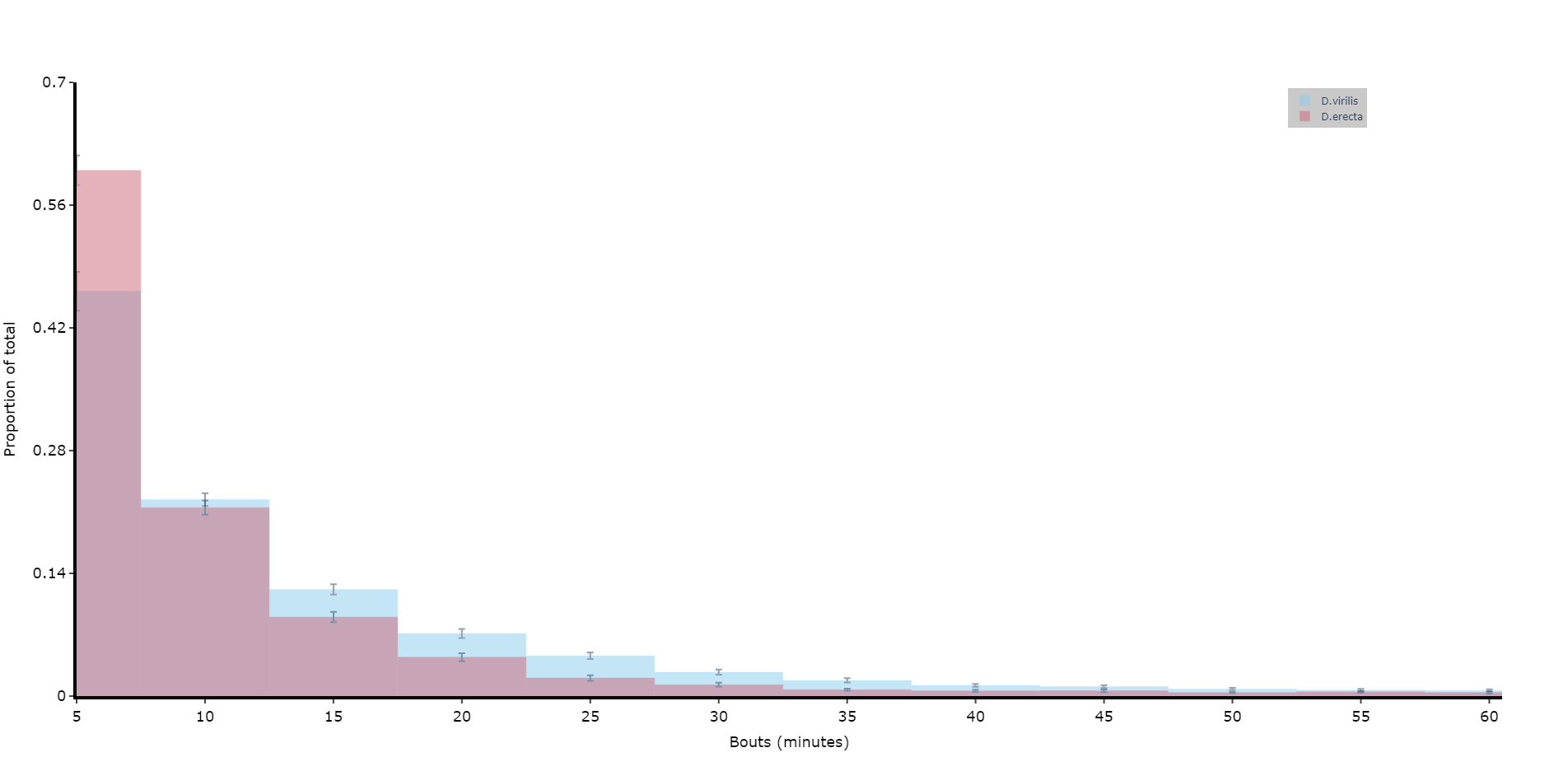
# You can take the output from above and create your own histograms, or you can use this handy method to plot a historgram with error bars from across your specimens
# Like all functions you can facet by your metadata
# Here we'll compare two of the species and group the bouts into periods of 5 minutes, with up to 12 of them (1 hour)

df.plot_sleep_bouts(
    sleep_column = 'asleep',
    facet_col = 'species',
    facet_arg = ['D.vir', 'D.ere'],
    facet_labels = ['D.virilis', 'D.erecta'],
    bin_size = 5,
    max_bins = 12
)
Find bouts of sleep
# If you haven't already analysed the dataset to find periods of sleep,0
# but you do have a column containing the movement as True/False.
# Call this method to find contiguous bouts of sleep according to a minimum length

new_df = df.sleep_contiguous(time_window_length = 60, min_time_immobile = 300)
Sleep download functions as methods
# some of the download functions mentioned previously can be called as methods if the data wasn't previously analysed
# dont't call this method if your data was already analysed!
# If it's already analysed it will be missing columns needed for this metho

new_df = df.motion_detector(time_window_length = 60)